Annotating Imagery at Scale with GeoVisual Search

Introduction

In this blog, we will show how to go from zero data to thousands of annotated satellite images using the Descartes Labs GeoVisual Search tool. Often one of the most difficult steps when creating a new machine learning model is finding ground truth data that is relevant to the problem you are trying to solve, and representative of the data you will encounter in production. Many times this problem is made difficult by a lack of access to data, but on the Descartes Labs Platform, there are petabytes of global satellite imagery spanning decades in time across dozens of sensors. Even with access to this volume of imagery, our objects of interest may be spread across the globe - how do we create annotated imagery quickly?

Global data discovery is hard and time-consuming

We should spend a little more time explaining why identifying example data can be difficult and time-consuming, especially for satellite imagery. For starters, our object of interest can be distributed over a very large area. We can not search the entire land-mass of the Earth for these objects by hand, which is precisely why we want a model in the first place. Moreover, the training dataset we generate should contain many instances of our object of interest without too many irrelevant examples. Therefore, we can’t just draw a large box around an area we think contains our object of interest and sift through it later.

Second, we need to identify not just the obvious examples of our object of interest, but also the edge cases where the visual context surrounding the object is very different from the most common examples. This drives the complexity of the data annotation problem, finding hundreds of edge case examples is going to be vastly more difficult than finding 1000’s more typical examples.

Lastly, environmental effects can plague your efforts. For example, clouds are common in some regions, making it difficult to identify the relevant examples from image to image. Similarly, how to handle seasonal changes? Luckily, if you are using the Descartes Labs Platform, masking for clouds and aggregation of imagery by time period is very easy and the GVS tool uses imagery free of clouds and aggregated into a single seasonal composite.

Descartes Labs GeoVisual Search

GVS is fundamentally an image similarity search tool. The tool contains two different base maps with varying resolutions and global coverages that have been pre-processed to be cloud-free and contain composited imagery from within a particular season. The GVS tool breaks up the land surface into overlapping tiles, each of which has been fed into a Descartes Labs developed convolutional neural network trained to generate a feature vector that summarizes the image tile in a compact way. When a user clicks a tile, a nearest neighbor search is performed between that tile’s feature vector and all other tile vectors in the database, with the k most similar neighbors returned to the user. For a more detailed explanation of GVS implementation, refer to Keisler et al, 2019.

When GVS returns the k most similar neighbors, it isn’t returning an image to be downloaded. Instead, GVS is defining the locations on the Earth where visually similar features were found. These locations are uniquely defined using a code (described later) which can then be used to generate images on the Descartes Labs Platform. In addition to the GUI-based GVS, the service can also be accessed programmatically which allows your GVS workflow to integrate directly with the other portions of your project.

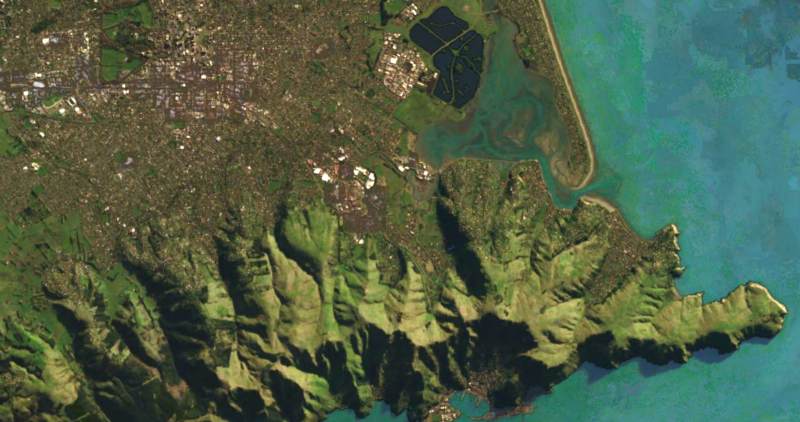
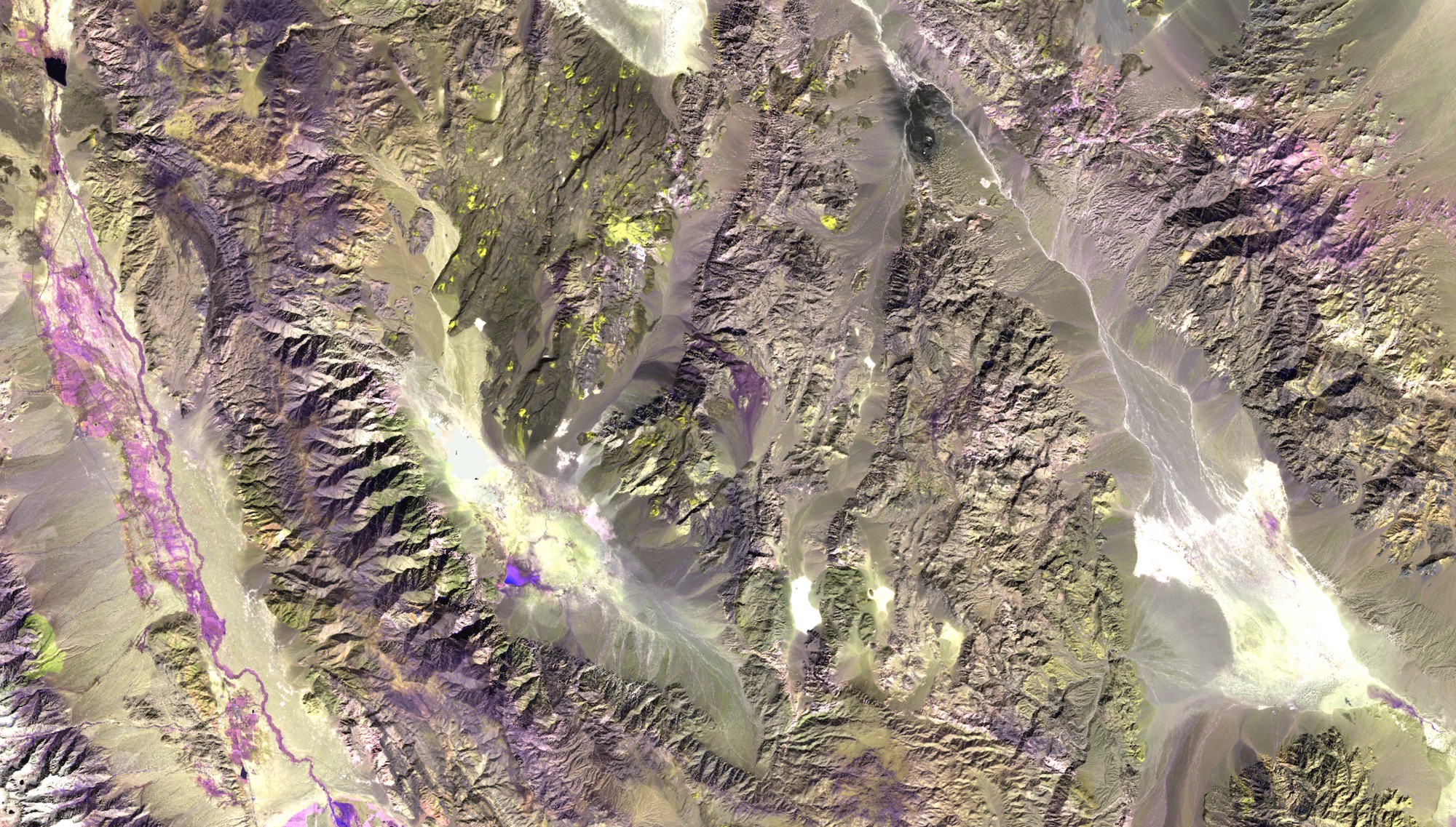
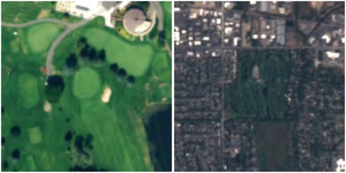
The types of features that can be leveraged by GVS depend on a couple of factors. One of these factors is the resolution of the imagery which dictates what features get resolved. The two imagery sources currently included in GVS are NAIP 1m imagery and Landsat 8 15m imagery. The second important factor is the size of the tiles that have been preprocessed. For both imagery sources, the tile size in pixels is the same at 128 pixels, however, the geographical area covered by each differs by nearly 200%. Therefore, a 128x128 pixel tile in the NAIP imagery might include a golf green and a few sand traps, whereas the same tile in the Landsat imagery will cover the entire golf course. This combination of resolution and tile size determines the types of features that can be found by GVS. Note however that nothing is stopping other imagery sources and different tile sizes from being added to the GVS tool.

Center Pivots Example

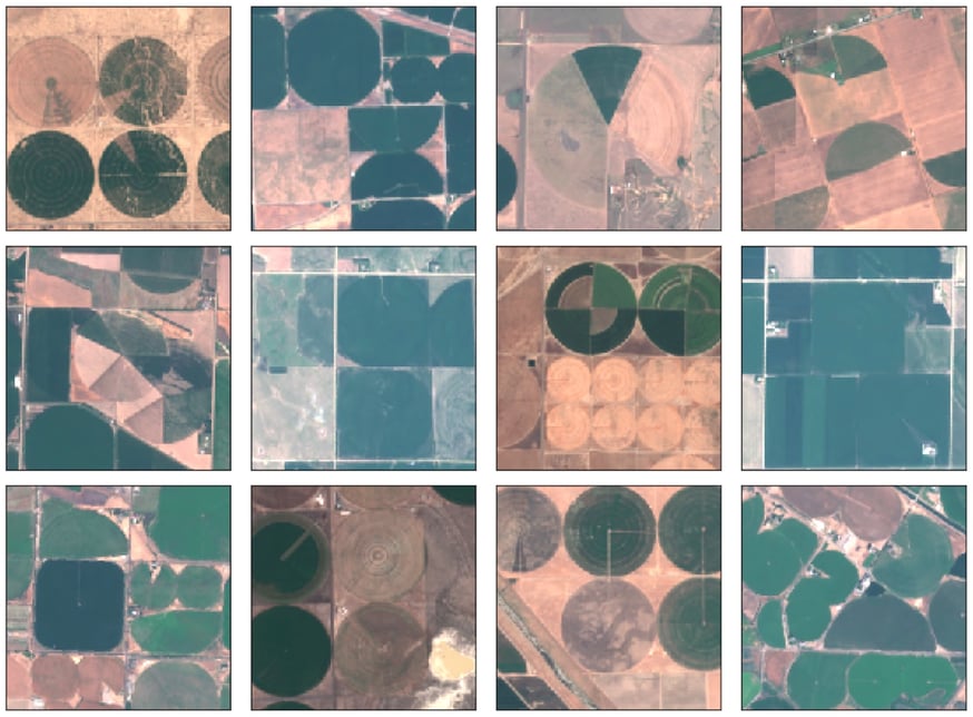
To illustrate how GVS can help with Data Discovery, we are going to show a use case that Descartes Labs recently developed to identify center-pivot irrigation fields in satellite imagery. A center-pivot irrigation system utilizes a central fulcrum from which a long pipe extends outward into the field. Along the main pipe, sprinkler heads are evenly spaced and provide uniform and direct water to the crops below them. During operation, the center-pivot system rotates about the central fulcrum providing water throughout the field in a circular manner. Due to this watering pattern, center-pivot fields often appear circular in satellite imagery which differentiates them from other types of agricultural fields. We want to automate the detection of this type of field using satellite imagery and a deep learning model, but we need thousands of examples to get started.

First, we need to select a number of initial tiles to use as input into the GVS tool. We can do this by browsing around in the GVS user interface. An important part of this step is finding and including a few edge cases. If you don’t include edge cases in this step, your training dataset will be mostly void of them. When you click in the GVS tool, the URL of the website changes and includes a snippet called dlkey with a unique identifier after the equals sign. The identifier looks like this: “64_32_15.0_13_2_4571” where each number separated by an underscore corresponds to “tilesize_pad_resolution_utmzone_utmx_utmy”. This code uniquely identifies that location on the Earth and can be used in the Descartes Labs Platform to generate a geocontext of exactly that area. So during this first step, we should identify ~30 initial tiles and record the dlkey code for each into a text document.

In the next step, we programmatically access GVS and query the tool for each template, keeping the first 60 results from each search. The results returned from the tool are more tile keys that we would store in a list. The last step is using those tile keys to generate images using the Descartes Labs Platform. Since the GVS tool returns a geographic area and not an image, we can generate images using any Catalog product we want, thereby changing how well resolved the features are for example, and sampling the object in images taken at different times.

When used in practice, we were able to turn ~35 templates into ~10,000 examples of center pivots across ~2000 images. This entire process takes less than an hour to complete and allowed us to move on to data annotation very quickly.

Data Annotation

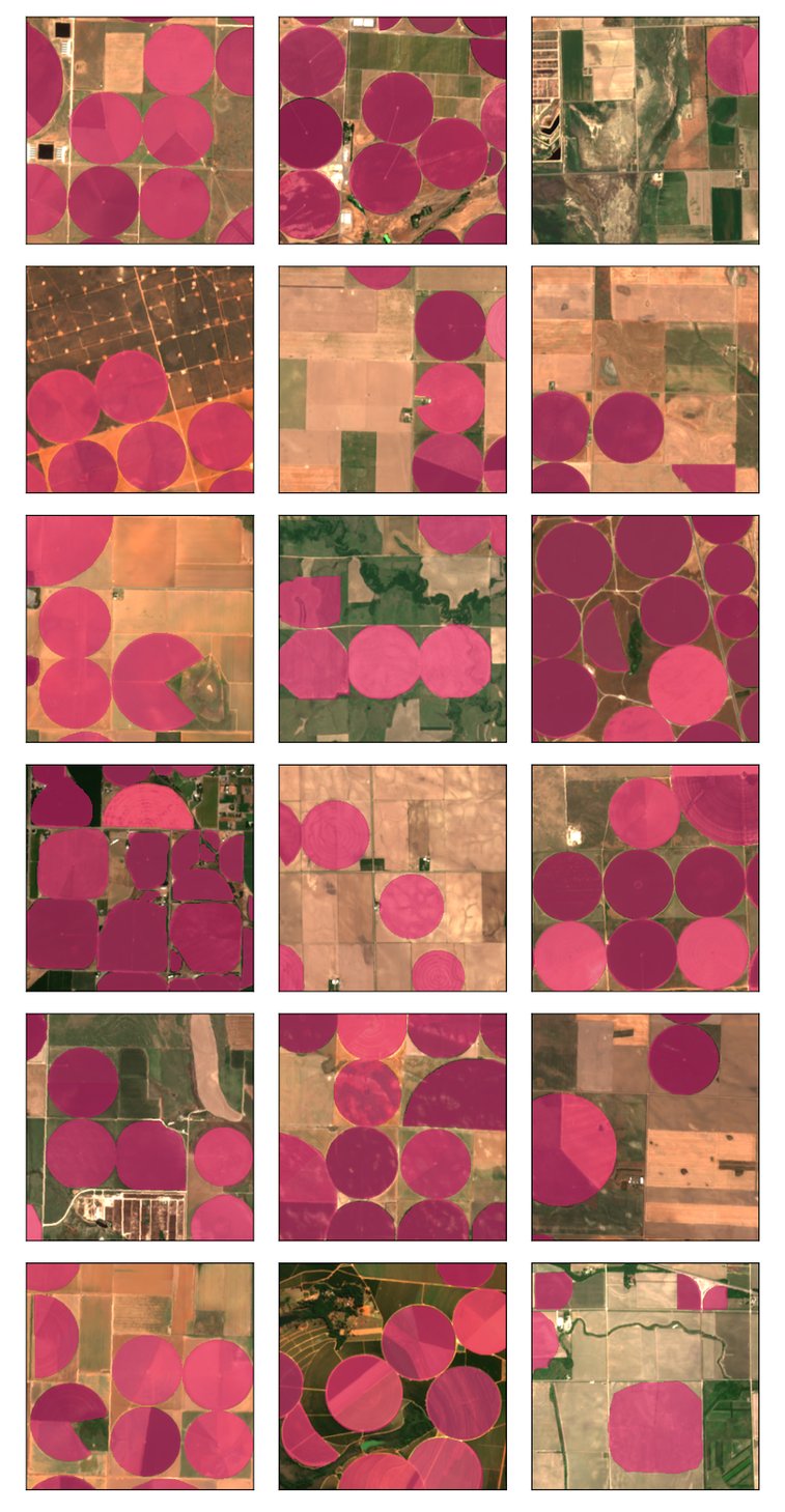
Now that we have thousands of images potentially containing center pivots, we need to quickly annotate these data before we can train a model. Luckily there are many companies that provide annotation services that can annotate these data in a matter of weeks. Descartes Labs uses CloudFactory + Dataloop for annotation services and their teams were able to annotate the center pivot data in ~3.5 weeks.

Below are some examples of labeled images where center-pivots are denoted as a red mask.

Conclusion

In this blog, we have shown you how to leverage Descartes Labs GVS tool to generate large training datasets for machine learning problems and also how to annotate the data very quickly. The combination of global search plus the Descartes Labs Platform is powerful, allowing us to do even more interesting things like finding objects in multi-spectral imagery with GVS and using the resulting geocontexts to generate images from other modalities in our Catalog like Synthetic Aperture Radar (SAR). If you would like more information about GVS and/or the Descartes Labs Platform, please visit our website to get in touch.

References

Keisler, R., Skillman, S. W., Gonnabathula, S., Poehnelt, J., Rudelis, X., &; Warren, M. S. (2019). Visual search over billions of aerial and satellite images. Computer Vision and Image Understanding, 187, 102790. https://doi.org/10.1016/j.cviu.2019.07.010