GeoVisual Search: Using Computer Vision to Explore the Earth

Last summer a group of artists and coders created Terrapattern, a ground-breaking demonstration of visual search over satellite imagery. We loved it. The demo aligned with many ideas we had been kicking around at Descartes Labs, and it was great to see somebody just go out and do it. It got us thinking about how we could extend visual search beyond cities, out to entire countries, or even the whole world.

Today we’re sharing our own demonstration of this technology, GeoVisual Search. The basic idea is:

• divide the earth’s surface into small, overlapping images;
• extract a “visual feature vector” from each image using a convolutional neural network;
• given a query image, search for “visual neighbors” in this feature space.

Let’s dive into some of the technical details.

Imagery

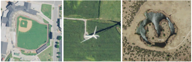
We’re searching over two imagery sources:

• Aerial over USA — We’re using 1-meter imagery from the National Aerial Imagery Program (NAIP) and the Texas Orthoimagery Program, with coverage of the lower 48 states.
• Landsat 8 over Earth — We recently made a 15-meter global composite using all data from Landsat 8, the jewel of NASA’s earth observation program.

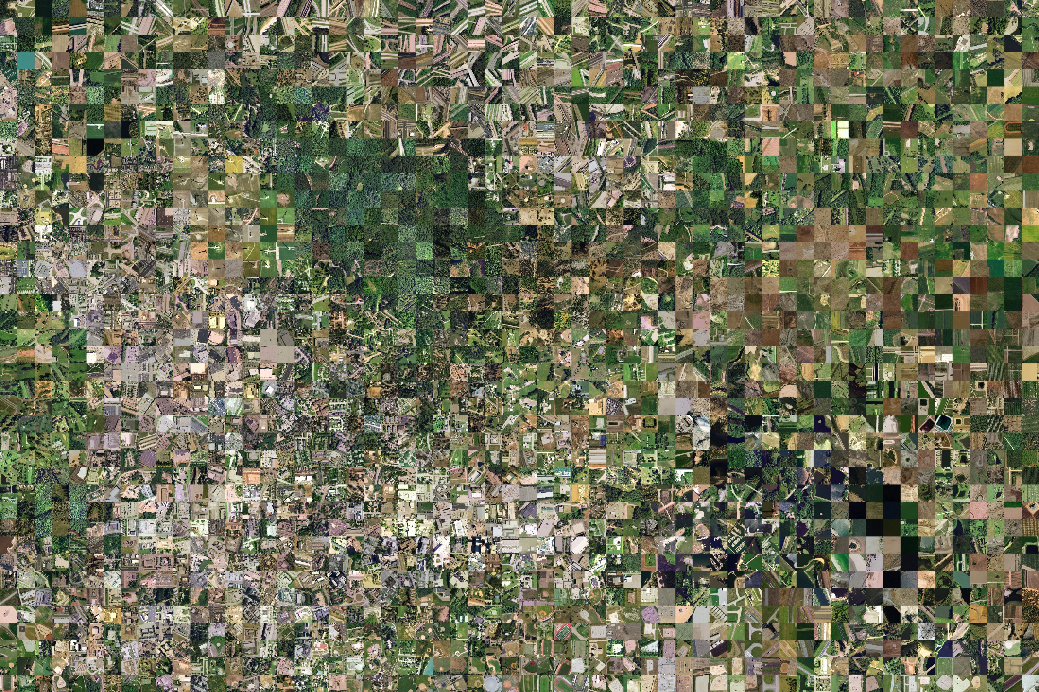
We used RGB imagery here, but the techniques generalize to other wavelengths of light, like infrared or SAR, or to more than three bands. We chop this imagery into small, overlapping tiles, 128 pixels on a side, and get to work generating features.

Features

We start with a 50-layer ResNet architecture, pre-trained on Imagenet, all conveniently provided by the Keras deep learning package. It looks like this 34-layer ResNet, only longer:

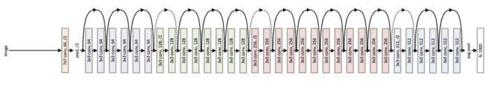
We initially experimented with the features generated in the last few layers of the Imagenet-trained net. These layers work surprisingly well with satellite imagery, despite being trained on images of cats and dogs, but we ended up making a couple of changes:

Binary Features — We decided that we ultimately wanted to search over binary features, due to their smaller memory footprint. To that end, we encouraged the net to make features very close to 0.0 or 1.0 at the layer of interest by injecting noise (during training) with an amplitude comparable to the width of the layer’s activation function. The net learns to make almost-binary features at this layer — otherwise the noise destroys the information that the layer is trying to pass on. Finally, we binarize the floating-point features by thresholding at 0.5.

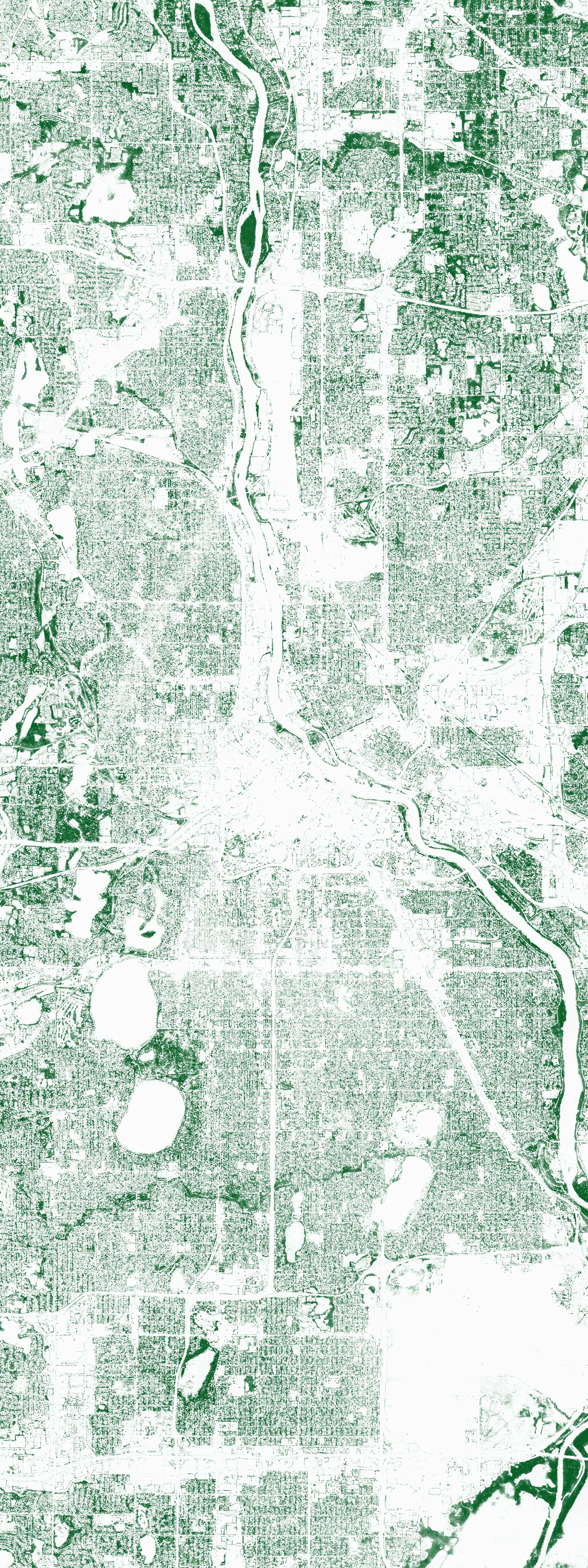
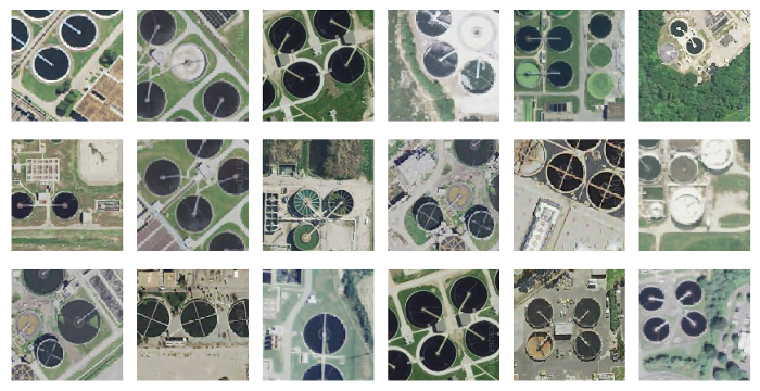
Customizing for Satellite Imagery — We customized this net to work with each source of satellite imagery. For NAIP, we followed Terrapattern’s lead and finetuned the net to classify into approximately 100 OpenStreetMap (OSM) classes, like parking lots or golf courses. We ended up adding a couple of fully connected layers and extracting 512 binary features from one of them. For Landsat 8, the OSM classes were less useful, so we instead used an autoencoder to compress the original 2048 floating-point Imagenet features into 512 binary features.

At the end of this process, we have mapped 393216 bits (the original 128x128x3 image) to 512 bits (the feature vector). These features form a compact representation of the visual information present in each image.

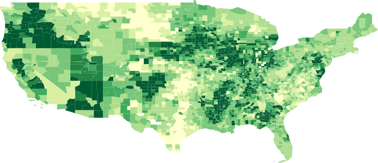
We pre-compute the feature vectors for all of the tiles in each dataset: about 2 billion tiles for NAIP and about 200 million tiles for Landsat 8. We distributed this computation across tens of thousands of CPUs in the Google Cloud Platform.

Search

Now that we have feature vectors, how do we search for similar vectors?

We first define a distance between vectors: the number of bits that differ, aka the Hamming distance. A small distance implies visual similarity.

Next we need to find the k nearest vectors to a query vector. We use two methods:

• Direct Search — By taking advantage of low-level instructions for comparing bytes and counting bits, we can do a direct, brute-force search over 200 million images in about 2 seconds. This solution works for the Landsat 8 dataset, which has about 200 million images.
• Hash-based Search — The NAIP dataset has about 2 billion images, and while the direct search works here, it’s too slow for interactive use. Instead we use an approximate method, bit sampling, which is a simple form of locality-sensitive hashing. More specifically, we use a family of 32 hash functions, each of which probes 16 bits of the full 512-bit feature vector. Each hash function returns a bucket of candidate neighbors, and we run a brute force search on the full (but relatively small) list of candidates. We store the hash tables in Google Cloud Bigtable, and the search takes about 0.1 seconds.

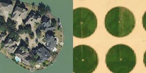
The result of all this: you click on some piece of the earth, and we return similar images in about one second. Try it!

Those are the main pieces of GeoVisual Search, but there is so much tech working behind the scenes that we didn’t cover here: our imagery pipeline, our python API for accessing this imagery, our custom virtual file system for cloud object storage, the auto-scaled map servers, the user interface, and more. Watch our tech blog for future posts.

This has been a really fun project to work on, one that has sent us into new directions for applying computer vision to satellite imagery at scale. Stay tuned for more, and if you think you might want to join our team, we’re hiring!