Article category: Mining, Science & Technology
Sentinel-1 Technical Series Part 2 | SAR Geocoding: Working...
In this post, we will describe Descartes Labs' SAR geocoding approach, which powers our global...
By Terry Conlon — Ph.D. Student in the Sustainable Engineering Lab at Columbia University. Terry completed the following work as a Descartes Labs intern this summer, where he worked with Rose Rustowicz to apply deep learning methods to timeseries of satellite imagery.
Despite numerous advances in the collection and distribution of satellite imagery — including those that allow sensing at sub-meter resolutions, rapid orbital periods, and public access to petabytes of data — one fundamental problem remains: how do you deal with clouds? In many parts of the world, persistent cloud cover prevents reliable information extraction from optical imagery, rendering many monitoring efforts dead on arrival.
Even though image contamination from clouds is both inevitable and ubiquitous, there is one silver lining: Cloud-cover does not impact all satellite imagery products! Certain data collected from radar sensors, such as those aboard the Sentinel-1 satellites, are not meaningfully affected by weather. As a result, scientists have been experimenting with methods of transforming non-cloudy radar images into optical ones, using advances in deep learning to extract hidden relationships between datasets: Recent papers have explored using either Sentinel-1 synthetic aperture radar (SAR) or interferometric synthetic aperture radar (InSAR) data layers to monitor vegetation phenology [Frison et al. (2018)], map crop types [Mestre-Quereda et al. (2020)], and generate optical imagery [Schmitt, Hughes, & Zhu (2018); Toriya, Dewan, & Kitahara (2019)].
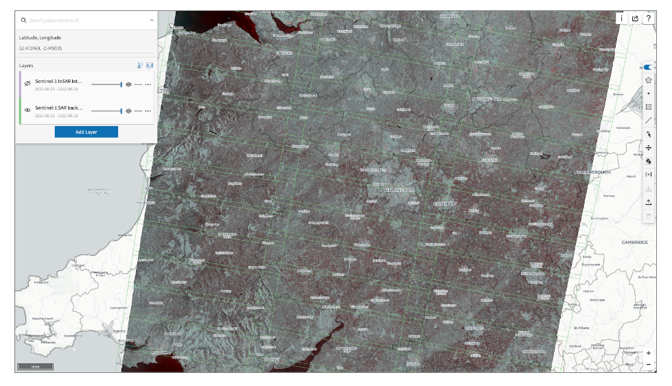
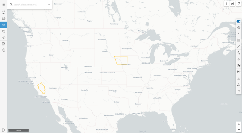
At Descartes Labs, I built upon this work over the summer, using both SAR and InSAR timeseries to predict vegetation indices (VI) in a region surrounding Fresno, California, and across an area of the Great Plains that enclosed portions of Iowa, Nebraska, and South Dakota; the exact boundaries of these regions are shown in Figure 1.
SAR measures two-dimensional surface backscattering, whereby polarized radar waves are transmitted onto a target, and the return waves are collected and recorded. On the Sentinel-1 mission, satellites emit vertically polarized waves and receive waves of both horizontal (denoted vh) and vertical polarizations (denoted vv). Reflection off vegetated surfaces can cause vertically polarized radar waves to return horizontally polarized (vh), although this process is highly dependent on the type of vegetation and its growth stage.
By comparing SAR backscatter measurements taken on two separate satellite passes, scientists can create an InSAR interferogram. The coherence layer of an interferogram measures the consistency of the scattering processes in the two SAR collects. Surface cover land types that demonstrate little change over time, such as buildings or pavement, will display high coherence; land cover types that produce different amounts of backscatter due to changing surface geometry will display low coherence values. Vegetation falls in this second category: Due to weather conditions or growth, leaves and branches can move by many wavelengths between passes, resulting in varying levels of backscatter over time.
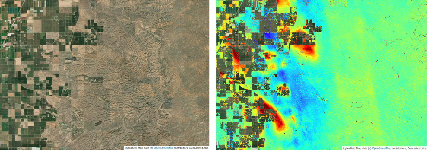
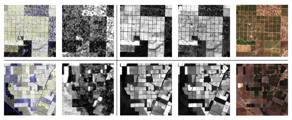
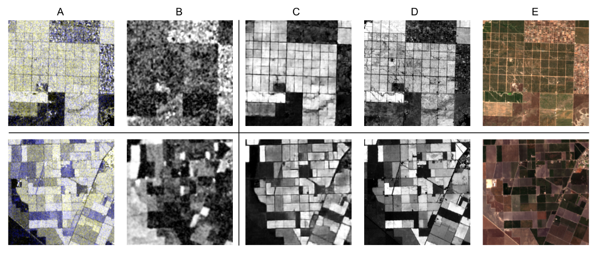
SAR and InSAR coherence layers, neither of which are appreciably affected by cloud cover, are shown in the first two columns of Figure 2. Column A presents vh backscatter in the red and green bands of the images and vv backscatter in the blue band; accordingly, pixels with high vh values look yellow and pixels over land cover types that do not change the polarization of the radar signal appear blue. Column B shows InSAR coherence: low coherence pixels are darker than their high coherence counterparts. In both displayed scene settings, we see alignment between the vh backscatter layers in Column A, the pixels with low coherence values in Column B, and the Sentinel-2 derived normalized difference vegetation index (NDVI) layer, which is presented in Column D. For reference, Column E presents the settings in true color RGB. Column C shows our NDVI predictions, generated with a modified Pix2Pix generative adversarial network (GAN), which is discussed in detail below.
Since their introduction in 2014, researchers have used GANs for a variety of different image generation tasks. In the case of paired image translation — a type of transformation that leverages the same image in multiple domains to extract cross-domain mappings — the Pix2Pix GAN architecture has successfully learned transformations in multiple use cases [Isola et al. 2017]. As our objective involved translating radar imagery into its optical counterpart, we modified a Pix2Pix to serve as our prediction model.
Our modified Pix2Pix used timeseries of SAR backscatter and InSAR coherence, along with Shuttle Radar Topography Mission slope measurements, as model inputs; it used Sentinel-2 derived VIs as targets. The input timeseries consisted of 4 timesteps (t’ = t .. t-3) 12 days apart, a duration which corresponds to the orbital period of a single Sentinel-1 satellite on a single ascending or descending pass. Similarly, coherence was calculated from Sentinel-1 passes 12 days apart. Input SAR timeseries were coregistered, spatiotemporally denoised, and converted to log-space; target VI layers (at time t’ = t) were clipped to the non-negative portion of their physical range. All input and target data were collected and organized with the Descartes Labs Platform.
We made an important modification to the baseline Pix2Pix training configuration in the form of an L1 crop loss: a loss proportional to the absolute difference between target values and predictions over cropland, determined by the USDA Cropland Data Layer. We imposed this loss to incentivize accurate predictions over cropland, as we felt that these were more important than predictions over non-cropped surfaces.
Predictions of enhanced vegetation index (EVI) using radar imagery, along with derived EVI from the Sentinel-2 images closest to them in time, are shown in the GIF below.
We can see in this GIF an overall alignment between our predictions and the VIs that would be expected at that time of year: Crops in Iowa cycle annually, with growth beginning after May and continuing through the summer until harvest around October. We also see a number of Sentinel-2 scenes where cloud cover renders the image meaningless. In these cases, our predictions provide information that is otherwise unavailable.
More generally, we have five primary findings from our work:
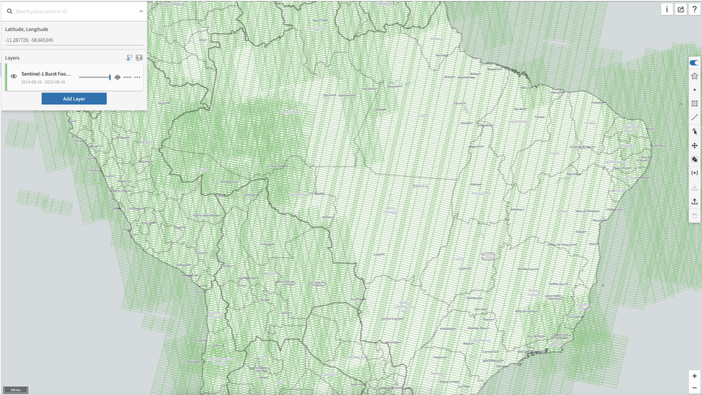
With the Descartes Labs Platform, we were also able to save our predictions for future retrieval, accessing them as we would for any other satellite imagery product. Figure 4 shows an example of how to retrieve predicted VI layers aggregated over a hand-drawn geometry and inspect the resultant timeseries, all in a Jupyter notebook.
In this GIF, VI predictions are shown for the yellow AOI. After selecting a portion of this region using a drawing tool, we can see VI predictions and Sentinel-2 derived measurements compared side-by-side.
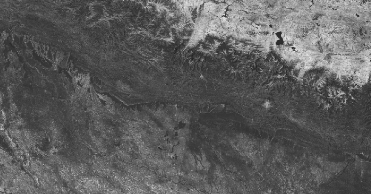
While the results shown here demonstrate a baseline ability to convert radar imagery into vegetation indices, other aspects of the translation process deserve further attention. Future work should investigate model transferability: Can one trained model be applied in numerous settings, or is location-specific training required? Furthermore, these translation models will provide greater value if they can be reliably deployed over topographically complex terrain. By focusing on these open questions, researchers have the opportunity to solve one of remote sensing’s fundamental problems: how to see through the clouds that occlude optical imagery.
Thanks Terry! Stay tuned for more featured work by our scientists, interns, and users.
Check out our platform page, view our webinar or drop us a line to discuss how the Descartes Labs Platform can help accelerate your work.