SAR Technical Series Part 4 | Sentinel-1 global velocity layer: Using global InSAR at scale

This is Part 4 of a technical series focusing on Descartes Labs’ global SAR processing capabilities. SAR provides a valuable remote sensing tool, and this series will dive into detail about how we process SAR data globally and build SAR and InSAR-derived products. Prior articles in this series can be found here: Overview, Part 1, Part 2, and Part 3.

Introduction

In this post we demonstrate how the interferometric products described in Part 3 can be used to build a global geospatial data product that assesses where the surface of the Earth is deforming. This data product can easily detect deformation rates of centimeters per year.

What is being measured and why

The surface of the Earth moves, sometimes due to geologic forces and sometimes in response to human activity. Aside from events like earthquakes, volcanic eruptions, and constructing or demolishing infrastructure, this motion is often quite slow. Examples of this motion include seismic creep along a fault, surface subsidence due to aquifer depletion or underground mining, uplift due to fluid injection from hydraulic fracturing, mine tailings compaction, and large human-made structures settling.

Measurements of this gradual motion can be a valuable diagnostic tool for man-made structures, and can provide an understanding of surface and subsurface activity.

How it is measured

An interferogram is a measure of change between two SAR images, and contains two data layers or bands. The first band is phase. The phase of a pixel in an interferogram has two contributors. The first is the change in effective round-trip distance between the satellite and the corresponding portion of ground, modulo the microwave wavelength. The second arises from changes, from one image to the next, in the scattering processes on the ground associated with that pixel.

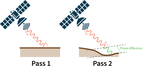
The effective round-trip distance is the geometric round trip distance combined with atmospheric effects such as tropospheric moisture. The geometric round trip distance can be estimated using orbit data and a digital elevation model (DEM). While the error in this estimate and the atmospheric effects are larger than the accuracy we seek, these errors and unwanted contributions are all nearly constant over small spatial extents. For this reason the appropriate quantity to work with is the phase difference between nearby points, where a value other than zero indicates one point moved relative to the other, provided that the phase from the scattering process didn’t change.

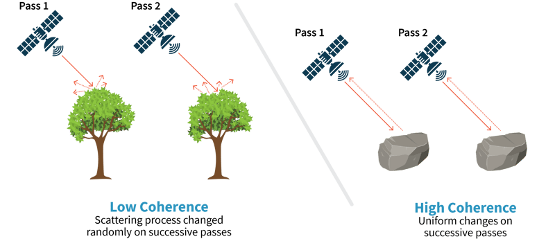
The second layer or band in an interferogram is coherence, which estimates whether the phase from the scattering process changed between collections. This estimation assesses the change in phase in a neighborhood of each pixel. If the phase change is nearly constant, coherence is high (close to 1) indicating that the phase came from changes in effective round-trip distance. Again, we assume that such a phase contribution affects the pixels in the neighborhood nearly uniformly. If the phase change is nearly random, the coherence is low (close to 0) suggesting that the scattering process changed for each individual pixel within the neighborhood in an uncorrelated way. In this case, we assume the phase difference is not indicative of the change in effective round-trip distance.

To ground this concept of coherence, we present some examples. Large swaths of exposed rock have high coherence. Vegetation has low coherence, as leaves will move by many wavelengths between image collections and this change will not  be correlated from one pixel to the next. Urban areas with human-made structures often have high coherence. An interferogram that combines SAR images before and after a landslide has low coherence.

The method we use for this work is a simplification of what is presented here and proceeds by partitioning the data into 10km by 10km tiles and for each tile:

1. We select all pixels with high coherence (above 0.6).
2. We form a triangulation of all these pixels and extract edges of the triangles as links.
3. For each link in this mesh, we consider the phase difference across this link for every available interferogram.
4. We attempt to match these link phases with a model parameterized by a constant line-of-sight (LOS) velocity and a term to account for any errors in the DEM. Selecting the values for the parameters is a per-link optimization problem, which runs quickly.
5. Once we have estimated the differential LOS velocity across each link, we estimate the point-based LOS velocity with a least-squares solve. This step is akin to integrating spatial differences to recover point values.

Systematic error contributions, e.g. phase gradients from orbit errors, that we assumed were sufficiently small to allow us to recover differential link velocity from model optimization in step 4, will likely accumulate in step 5. To address this, we detrend each tile. We fit the data to a bilinear surface, and subtract that best fit from the data.

Finally, we average data on tile overlaps to reduce seam artifacts at tile boundaries.

The resulting data capture the LOS deformation rate of each point relative to the surrounding points. If there is a large spatial trend that is constant or linear across an entire tile it will be removed when we detrend the tiles.

With a standard Descartes Labs user account, we used this method to generate an LOS velocity map for 2021 at a 20m posting for the Southwest US in a week.

What the results look like, and how to interpret them

For each of the results below we show optical imagery and LOS velocity measurements of the same location. Due to the constraints of SAR imagery, the LOS incidence vector is roughly 35 degrees off vertical.

Shopping plaza

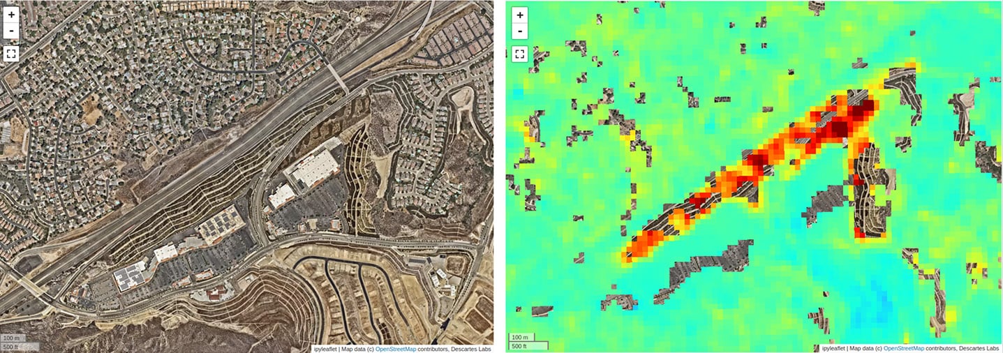
At a lat, lon of roughly 34.3956, -118.4638, there is a shopping plaza Southeast and up an embankment from the Antelope Valley Freeway in Santa Clarita, CA. Our data suggest a subsidence (e.g. motion away from the satellite) rate exceeding 5cm/year in places. The orange and red areas indicate the surface is moving away from the satellite at a faster rate than any of the surrounding area.

Interstate 80

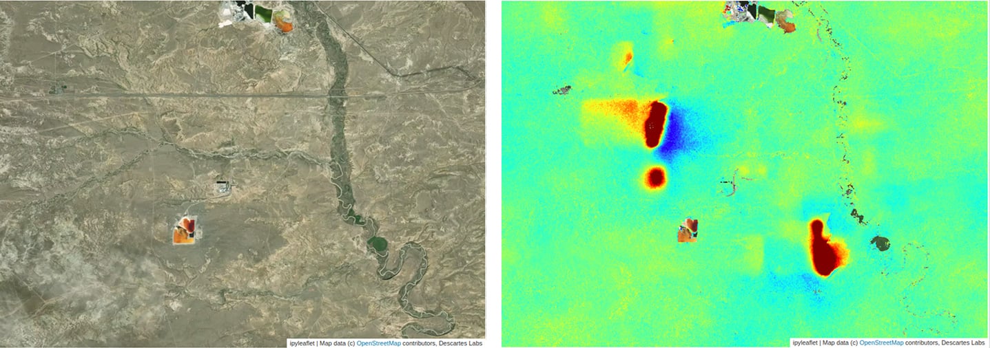
At a lat, lon of roughly 41.4910, -109.7630, south of Interstate 80 near Green River, WY, we see large subsiding areas, likely due to underground resource extraction.

Aquifer

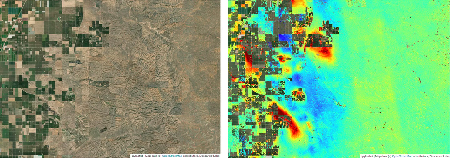
At a lat, lon of roughly 35.6666, -119.0338 we see subsidence likely due to water being drawn from an aquifer to support crops outside of Mcfarland, CA. Note that active farm land leads to vegetation, which drives coherence below 0.6, preventing us from making a measurement over the green crops.

Oil fields

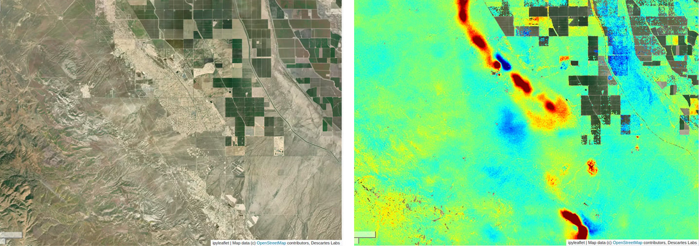
At a lat, lon of roughly 35.4342, -119.7172 we see subsidence and uplift at oil fields near Missouri Triangle, CA, likely due to both resource extraction and ground water injection.

Conclusions

Having stacks of preprocessed interferograms enables us to rapidly build a LOS velocity map anywhere in the world, using appropriate algorithms. Such a map allows InSAR to be a queueing mechanism where we can simply pan around to identify regions that may deserve more attention. A global velocity map enables an effortless “first look” that speeds analysis. We’ll present a more detailed assessment in the next part of this series.

💡 Interested in using this technology?

Contact our team to discuss how we can integrate our global InSAR product into your processes.

Check out the next post in this series, "Global scale InSAR", where we focus on the salient features of our global InSAR pipeline.

Reference:
Agram PS, Warren MS, Calef MT, Arko SA. An Efficient Global Scale Sentinel-1 Radar Backscatter and Interferometric Processing System. Remote Sensing. 2022; 14(15):3524. https://doi.org/10.3390/rs1415352