Article category: Mining, Science & Technology
SAR Technical Series Part 4 | Sentinel-1 global velocity...
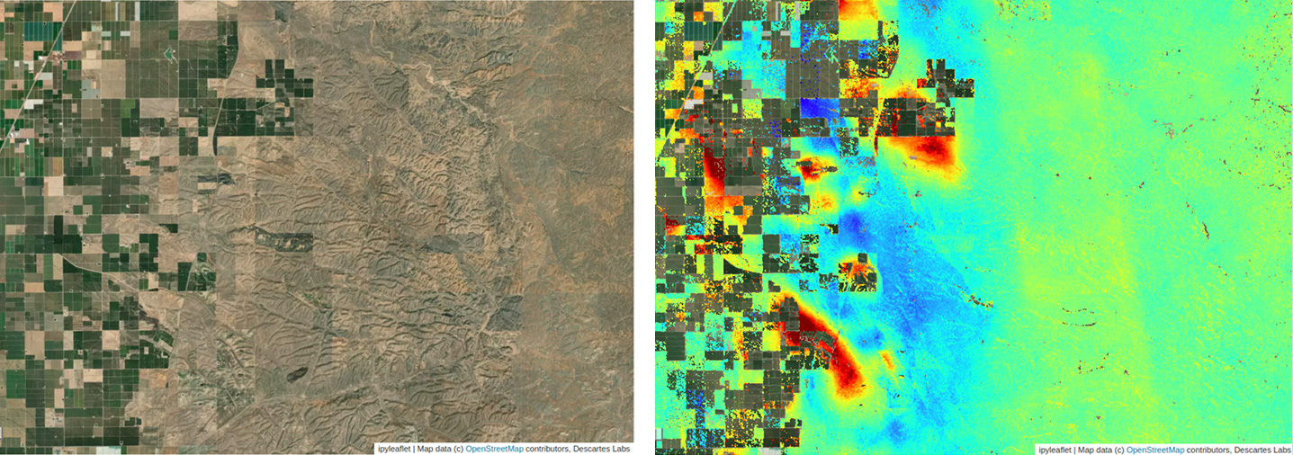
Descartes Labs uses interferometric products to a build global geospatial data product that detects...
This is Part 2 of a technical series focusing on Descartes Labs’ global SAR processing capabilities. SAR provides a valuable remote sensing tool, and this series will dive into detail about how we process SAR data globally and build SAR and InSAR-derived products. The prior two articles in this series can be found here: Overview and Part 1.
In Part 1 of this series, we described the fast data access mechanisms for Sentinel-1 SAR data. In this post, we will describe Descartes Labs’ SAR geocoding approach, which powers our global scale pipelines. We will present this in terms of well known GIS concepts, in hope that this will assist in demystifying SAR data to users who are not familiar with this type of datasets and for future adopters of this technology.
Note, we will focus on the lowest level calibrated SAR products - Level-1 SLCs in this blog. Every SAR instrument is unique and we will not concern ourselves with calibration of data from each SAR source, as part of this blog. We assume that data providers release calibrated (to the best of their ability) SLC data. We will also focus on Sentinel-1, since this is the most widely used SAR dataset in the world and is freely available.
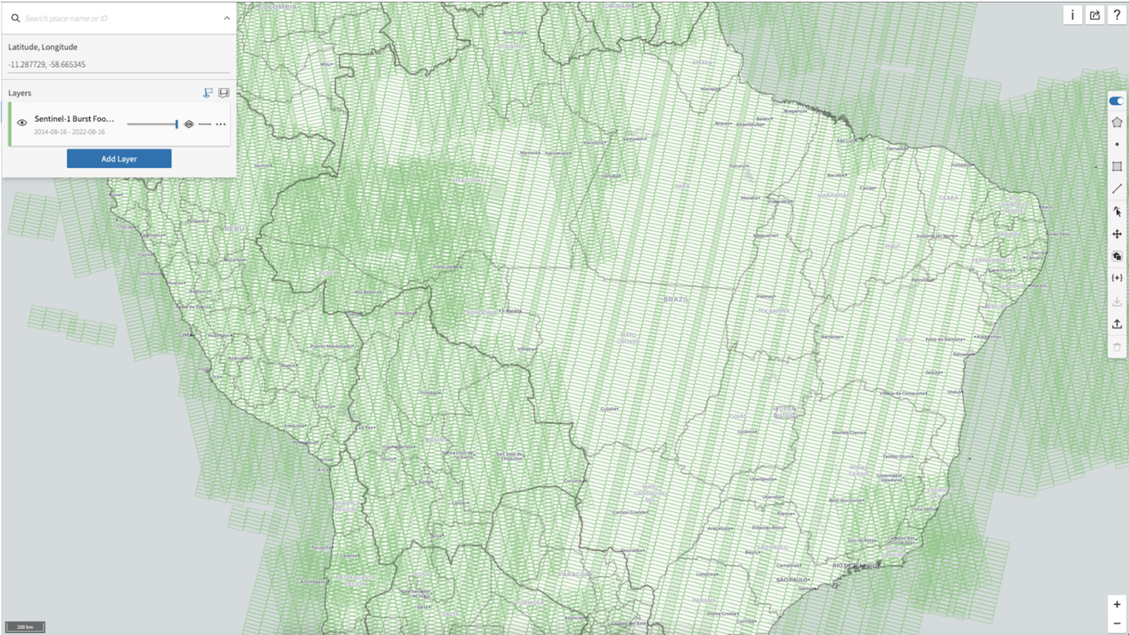
Sentinel-1 Level-1 SLC granules are organized as a collection of bursts (See Part 1). Each burst, though not very obvious to users working with optical datasets, has a well defined projection system. The primary challenge for GIS software to work with SAR data is that this projection cannot be represented simply by an EPSG code or a simple PROJ string. Hypothetically, if we were to write a PROJ string representation for a SAR SLC (Sentinel-1 burst), it would look something like:

The `zero-doppler` projection indicates that pixels are arranged in a grid that is tangential to the satellite’s orbit - the system used by Sentinel-1. Most commonly used SAR datasets – such as those generated by Sentinel-1, the TerraSAR-X constellation, the COSMO-SkyMed constellation, ICEYE, Capella, RISAT – all use the zero doppler system. The side argument indicates if the platform is looking left or right. The range argument indicates that the data is on a uniform slant range grid. There are other systems for distributing SAR imagery, which we won't discuss here. Note that a similar notation can probably be used to describe any of these other SAR projection systems. Also note that this is a 3D Coordinate Reference System (CRS), i.e, the coordinate transformation depends on altitude of the point.
The key takeaway from using this analogy is that any change in the projection parameters above essentially represents a different coordinate system. A direct consequence of this is that every SAR image, even if acquired over the same AOI, inherently has a different projection system since satellite orbits do not repeat perfectly. Note that the geolocation of points in the image needs the orbit information, which we have included above as a semi-colon separated list of time-tagged cartesian positions and velocities for simplicity. Often this information is read in from external orbit files or from metadata included with the radar imagery.
Similarly, the geotransform for a SAR SLC image that uses the projection system above would look something like:
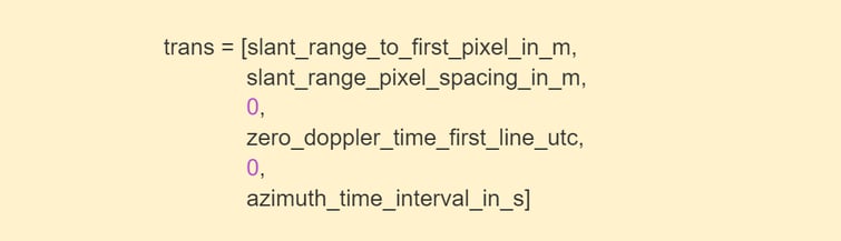
Most SAR satellites follow a polar orbit where the along-track time is roughly equivalent to the Y-coordinate/latitude and slant range from the satellite's orbit is roughly equivalent to the X-coordinate/longitude. A similar geotransform for GRD images would replace slant range with ground range in the notation above and the same interpretation still applies. Such a simplistic geotransform-like representation might not be applicable to custom SAR projection systems.
As described above, each SAR image is distributed in its own projection. Hence, coregistering one SAR image to another acquired over the same AOI is essentially a reprojection operation. A minor complication in this reprojection is the nature of SAR imaging itself. A SAR image represents a 2D representation of a 3D world - and we are trying to coregister two slightly different projections of the same underlying 3D world; akin to aligning photographs acquired from different perspectives. This is true of optical images as well, but SAR is essentially an off-nadir view often collected at an incidence angle of greater than 30 degrees. To allow us to align these images precisely, we rely on a model of the 3D world in the form of a digital elevation model (DEM).
Traditional approaches select the zero-doppler coordinate system of one image, which we will call the reference, and reproject the other images onto this reference zero-doppler coordinate system. This approach to reprojection is expensive and represents the core of any widely used SAR processing software, such as SNAP, ISCE, and GMTSAR. Additionally, this approach leads to a substantial amount of SAR imagery projected into the zero-doppler coordinate system of the reference Image. Imagery projected as such cannot be operated on with standard GIS tools. In contrast, one could choose a well known GIS coordinate system as the common projection system.
At Descartes Labs, we use a UTM system as the common projection system and project every image to this common system. This approach is computationally efficient as we eliminate the need for maps between different zero-doppler coordinate systems and we have optimized implementations for the map from geographic coordinates to zero-doppler coordinates on single CPUs. Since all the geocoded imagery is in a well known CRS, we are able to use the same set of data manipulation tools that we have developed for optical and other geospatial datasets. In a broad sense, we have reduced SAR geocoding to an enhanced `warp` operation with custom interpolators.
SAR images represent 2D projections of signals scattered from 3D terrain, and as such can also be interpreted as a point cloud. Representing SAR data as a raster is only a convenient method of data organization. Organizing SAR data in the original zero-doppler coordinate system has useful spectral properties, while organizing it in the UTM system significantly improves its interoperability with other datasets. The physical measurements themselves are associated with points in 3D space and pixels can be interpreted as a point cloud in radar geometry. Consequently,
Note that this reprojection operation has only been possible due to the substantial improvements in the quality of associated ancillary datasets and metadata in the SAR ecosystem in the last decade. Notably:
In geospatial data analytics, Equal Area or UTM CRSs are suited for data aggregation whereas LatLong systems are useful for other applications. The same concept also applies to SAR data. Native radar geometries (like our hypothetical projection system above) are best suited for spectral sub-banding (also known as sub-looking) and calibration operations; whereas transforming the data to well known CRS early in the chain allows us to leverage optimized data access mechanisms / representations with SAR data. This enables us to operationalize established applications like backscatter or InSAR analysis. Eventually, as long as the point cloud is oversampled in well known CRS an equivalent pixel-by-pixel geometric transformation can always be determined for computing additional useful parameters like incidence angles, interferometric baselines etc without loss of precision.
Our geocoding approach also enables consistency between suites of products derived from geocoded SLCs. SAR / InSAR workflows often involve a spatial averaging / decimation (also known as multi-looking) step to help alleviate speckle effects. In traditional, image-by-image processing approaches this decimation is often performed in original radar coordinates (e.g., generation of GRD from SLC) and then resampled onto a uniform grid. As shown in the figure below, this often leads to averaging of different segments on the ground in different projection systems and the differences can get further exaggerated in heterogeneous terrain.
This effect is understood within the InSAR community and one of the commonly used methods to alleviate this effect is to group acquisitions by satellite geometries and coregister every image in each group to a chosen reference image. This stacking approach significantly reduces phase closure artifacts in InSAR analysis compared to using interferograms that were generated pair-by-pair. Note that even in this case, the same issues resurface when comparing aggregated results across satellite tracks / geometry groups.
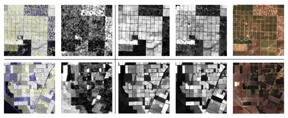
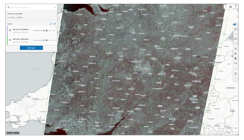
With Descartes Lab’s geocoding approach, since we geocode/warp at full resolution (oversample) and then aggregate on a standard grid, we achieve consistent spatial averaging even across imaging geometries. We thus ensure that the backscatter products and not just InSAR products benefit from such consistent processing as well. Our approach allows us to generate high quality global backscatter (10m) and InSAR (20m) datasets, on the same grid as Sentinel-2, that are very well coregistered on the live Sentinel-1 datastream from ESA. This is in fact how the recent SEN12TS dataset was generated. We currently are unaware of any other complementary backscatter and InSAR dataset with similar coregistration properties.
%20and%20InSAR%20coherence%20(Bottom).png?width=1211&name=Snapshot%20of%20Radar%20backscatter%20VV-VH-VH%20(Top)%20and%20InSAR%20coherence%20(Bottom).png)
In this post, we described Descartes Labs' approach to geocoding SAR data that powers its near real time Sentinel-1 based SAR backscatter and InSAR coherence pipelines. In the next post, we will dive deeper into our global InSAR product and into how we combine our fast data access mechanism (Part 1) and SAR geocoding (Part 2) into a global InSAR analytics product focused on real time monitoring.
Contact our team to discuss how we can integrate geocoded bursts into your processes.
Check out the next post in this series, "Global scale InSAR", where we focus on the salient features of our global InSAR pipeline.

Reference:
Agram PS, Warren MS, Calef MT, Arko SA. An Efficient Global Scale Sentinel-1 Radar Backscatter and Interferometric Processing System. Remote Sensing. 2022; 14(15):3524. https://doi.org/10.3390/rs14153524