Gaze into the Future with Downscaled Climate Models

The combination of global climate models and land cover data can be used to estimate the regional effects of climate change years into the future

By Sepideh Khajehei — Sepideh is an Applied Scientist at Descartes Labs working on the Forestry & Climate team. She has a Ph.D. in Civil and Environmental Engineering from Portland State University with domain expertise in hydrology, weather and climate risk, and natural hazard prediction. With collaboration by Alex Diamond, Julio Herrera Estrada, and Jason Schatz.

In December 2019, Goldman Sachs issued an environmental policy framework that halted the company’s financing of deals in environmentally damaging industry sectors. Carbon-intensive projects like coal-fired power generation, mountaintop removal mining, and arctic oil and gas exploration would be avoided in favor of projects that promoted mitigation, adaptation, and the advancement of “diverse, healthy natural resources — fresh water, oceans, air, forests, grasslands, and agro-systems.” Goldman’s decision became a tipping point in 2020 as other major banks quickly followed suit with similar policies.

After years of worsening financial losses from bad loans caught up in natural disasters and an accumulating string of accurate but foreboding climatic projections, the global financial system is starting to see the writing on the wall. Aside from the acute financial losses, the banks’ abrupt change in attitude is influenced partly by the science behind Global Climate Models (GCMs) and their costly projections of a future with unsustainable anthropogenic warming.

At the same time, many banks have started to pursue “climate-forward” strategies with the rise of ESG risk-factors in equity investing and shifting customer demographics and preferences that place a higher premium on mitigating systemic risks from climate change, pandemics, social unrest, and other existential threats.

Background on GCMs

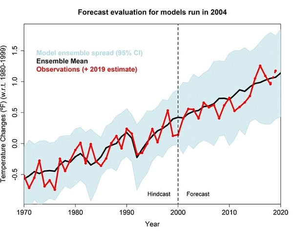
To understand the practical benefit of GCMs for climate change mitigation and adaptation efforts, we can look at how they are used by the Intergovernmental Panel on Climate Change (IPCC). The mission of the IPCC is “to provide the world with objective, scientific information relevant to understanding the scientific basis of the risk of human-induced climate change, its natural, political, and economic impacts and risks, and possible response options.”

One of the ways the IPCC accomplishes their mission is by leveraging the outcomes of the Coupled Model Intercomparison Project (CMIP), a global, collaborative experiment that compares how a set of climate models react under different greenhouse gas emission scenarios. These outcomes contribute to ongoing IPCC assessment reports that detail the effects of climate change and provide suggestions for mitigation and adaptation. The current IPCC sixth assessment report relies on an updated set of global climate modeling from CMIP6, the latest phase of the CMIP project. In CMIP6, these emission scenarios are called Shared Socioeconomic Pathways (SSPs), which are defined by different socioeconomic emission assumptions.

The uncertainty around climate projections is high, and in reality, no one knows exactly what will happen 20, 50, or 100 years in the future. Without understanding the actual choices humanity will make, GCMs can’t say for sure how much CO2 will be emitted into the atmosphere in the decades to come (hence why we derive projections and not forecasts from GCMs). However, we can use these scenarios in a proper manner, considering their relative likelihood, in order to prepare for future events and mitigate pessimistic scenarios as much as possible.

Fortunately, modern-day tools can expand the practical use of climate models by integrating regional geospatial data and scalable computing. The models can be “downscaled” to project the future effects of climate models onto regional geographies. This allows climatic scenario analysis to be performed over areas like cities, coastlines, forests, natural attractions, and parks, or any place that governments or businesses intend to use and extract value from in the future.

California Dreamin’

Let’s say you run a business that has staked a large percentage of your future cash flows on California’s agricultural industry. It’s critically important for you to understand what temperatures and precipitation are going to be like in 2030, 2050, and beyond. Those almond groves and dairy cows can’t fetch water for themselves after all.

With just a little bit of programming experience and a bit of documentation, you can produce your own downscaled climate analysis in just a few days. Let’s explore below.

Downscaling by Regional Land Cover

We’ll start by installing a Python library called Scikit-downscale in Workbench, Descartes Labs’ hosted JupyterLab environment. Scikit-downscale is an open-source toolkit for statistical downscaling developed by collaborators around the Pangeo project, “a community platform for Big Data geoscience.” By leveraging Pangeo’s integration with Google Cloud, we can access the CMIP6 model runs from Google Storage buckets in a blink of an eye.

Once the model runs are in hand, we’ll choose a training and predicting period and a region for downscaling (California) and then pick the appropriate CMIP6 historical and future model runs (SSP585). SSP585 is a shared socioeconomic pathway defined based on fossil-fueled economic development, where the main focus is the rapid growth of the global economy, resulting in an increase in the consumption of fossil fuel resources.

The downscaling process starts with reading the historical temperature simulations from the CMIP6 GCMs and corresponding observations from gridMET, a set of surface meteorological data suitable for this study due to its high spatial resolution (4 km). These data are loaded into the Xarray and Dask data structure using the same mapping coordinate system. Afterward, Scikit-downscale is called to train on the historical model runs. The Dask client is used to parallelize the workload over Descartes Labs’ available computational resources. Finally, the trained model is used to downscale the corresponding future scenario as shown in the graphic below.

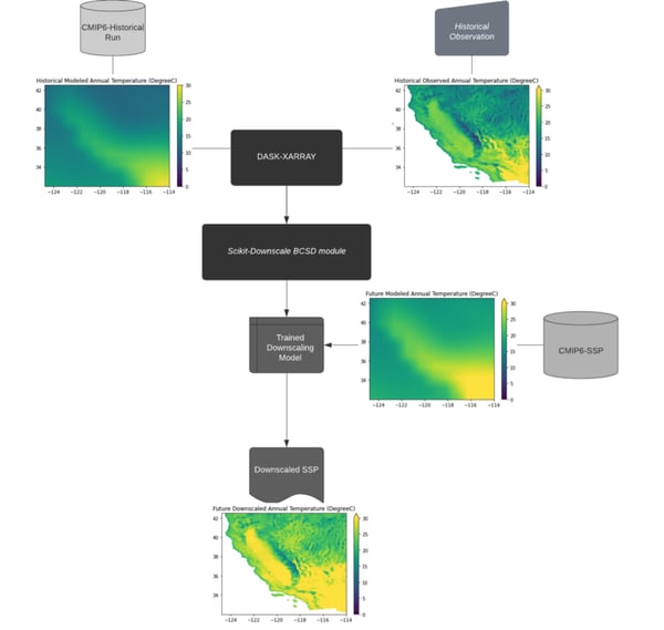
Once the downscaled model has been generated, the outputs can be ingested as data products in the Descartes Labs Catalog.

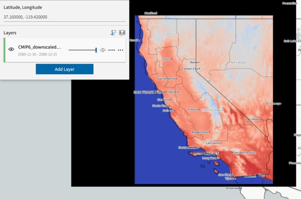
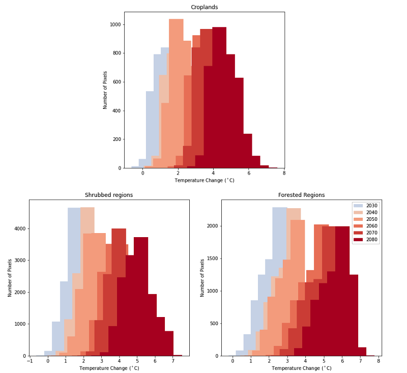
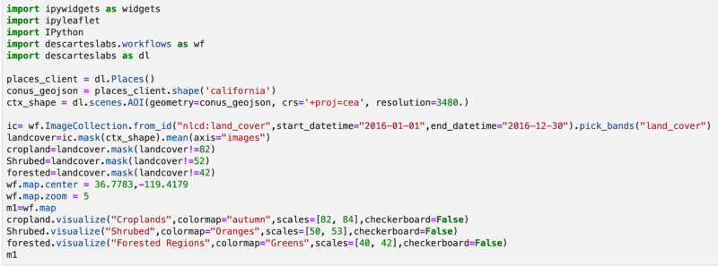
Now that the models have been loaded, we can combine them with other geospatial data to create statewide maps for more granular scenario analysis. For example, we can use them to investigate the projected increase in temperatures over different land cover types across the state of California. Using NLCD Land Cover data, we extract the areas with shrubs, forests, and croplands over California, which amount to most of the state’s land cover types.

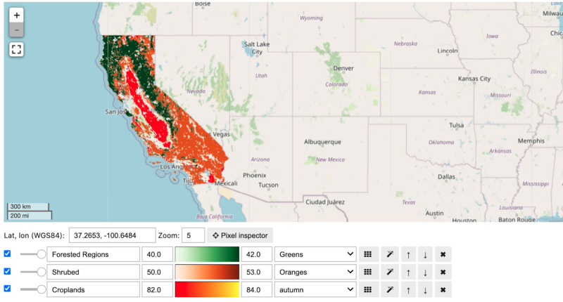
Using the land cover as a base layer, we can now calculate the decadal temperature changes using the downscaled climate outputs and 2018 temperature observation data across each decade from 2030 to 2090.

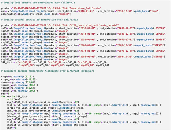
As a result of running the code above, we can generate decadal histograms of temperature change for each land cover type in California through the 2080s. The results are shown in the animated graphic below, with warming of approximately four to six degrees Celsius on average for each land cover type. We now have base maps that contain temperature estimates for each pixel, for the next 70 years!

Making the Complex Simple

Processing raster data like this across such massive geographies and timeframes is no simple task. What used to take weeks or months assembling all of the data, downscaling the GCMs, and converting all the other datasets into a common coordinate system now becomes a much simpler and faster process with these tools from Pangeo, Scikit-downscale, and the Descartes Labs Platform.

Thanks to Pangeo, we don’t have to worry about the data structure for the observation data and GCMs. And thanks to Scikit-downscale, generating downscaled products can be done in just one line of code. Finally, the Descartes Labs Platform allows us to orchestrate and process everything in one interface, meaning we can evaluate future temperature changes on a vast majority of assets and natural resources with our combination of downscaled products and geospatial data.

Moving Fast Toward Resiliency

Climate change is happening fast, so we have to move fast as well to mitigate it and adapt to its impacts. Instead of spending months downscaling the GCMs, converting to similar formats, storing everything together in a way that’s quickly accessible, and porting to new systems to visualize the data, we can tackle all of this in days and move on to make more informed decisions that build resilience in an uncertain future.

If you’d like to understand the effect of climate change on your asset, city, or region of interest, get in touch with us to learn how.

“All models are wrong, but some are useful” — George Box, prominent British statistician

Thanks, Sepideh! Stay tuned for more featured work by our scientists, interns, and users.

Check out our platform page, view our webinar, or drop us a line to discuss how Descartes Labs can help accelerate your climate analysis.