Article category: Mining
Get to Know Marigold (Part 7): Marigold Workflows & Derived...
In the conclusion to our Get to Know Marigold series, we compute a Principal Component Analysis,...
Article category: Mining
Welcome to Marigold! This is part 4 of our Get to Know Marigold blog series with helpful videos. Previous blog series can be found here. Part 1: Functionality and Processing Tools | Part 2: Introduction to the Bare Earth Composites | Part 3: Vegetation and Water Masking
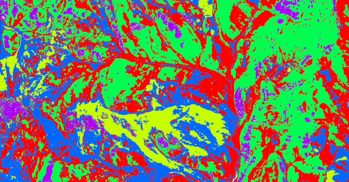
In the following video snippets, we will walk through how to use K-Means clustering to mask out areas you would like to remove from your imagery using the Descartes Labs’ Marigold software built-in capabilities.
When using an unsupervised classification like K-Means clustering in areas with complex surface cover, the first areas identified are often the groups of pixels that are most spectrally and statistically different from the rest of the data. Multiple stages of masking make it easier to identify and mask more subtle features. In this video, we use data that we previously masked for vegetation in another training video and apply a new shadow mask created through K-Means Clustering.
If you need a refresher on creating and applying Vegetation Masks, watch our training video on Vegetation Masking for those instructions.

K-Means clustering is an unsupervised classification algorithm that segments the input dataset into a "K" number of different clusters. From these clusters, areas that require masking can be identified, and then turned into mask layers to apply to datasets.
While the example in this video focuses on shadow, this technique can also be applied to areas of:
In this example, areas of topographic shadow are visibly obvious in the Sentinel-2 Bare Earth Composite. Shadows are areas that have very low reflectance values and therefore have a very different spectral response to the rest of the data. This makes it a perfect target for an unsupervised classification.
To create a K-Means cluster of this image:
Next, identify the number for the cluster group that you will turn into a mask, in this case the purple shadows.
Tip: Toggle off the Pixel Inspector to optimize Marigold’s performance speed.
Now you can create a shadow mask:
To apply this mask to a dataset of your choice, select the Apply Mask tool in your Processing Toolbox.
Then, choose the dataset you wish to mask, in this case the Sentinel-2 Bare Earth Composite data that we masked for vegetation in a previous training video.
Tip: Applying multiple masks to the same dataset will help to reduce multiple potential sources of false positives.
Next, select the mask you wish to apply to that data, in this case the shadow mask that we created. Provide the output with a name, and then click Mask Layer. By turning off other layers and changing the basemap, you will now see where your data has been masked, in this example removing the shadows from the imagery.
For any additional stages of masking using K-Means, we recommend that you re-run your K-Means clustering on the masked out data, following the previous steps in this video. This will identify more subtle groups for masking, since more statistically-significant pixels and groups have already been removed from the imagery.
Tip: Re-run your K-Means clustering on the masked out data to identify more subtle groups for masking.
You now know how to use an unsupervised classification technique to mask out shadows as well as other surface cover types. Once you have satisfactorily masked your data, you can use Marigold’s processing tools to identify lithologies, alteration, and mineralization with even greater confidence.
![]() In the next Get to Know Marigold blog, we'll show you how to create a series of standard multispectral derived products in Marigold.
In the next Get to Know Marigold blog, we'll show you how to create a series of standard multispectral derived products in Marigold.
Article category: Mining
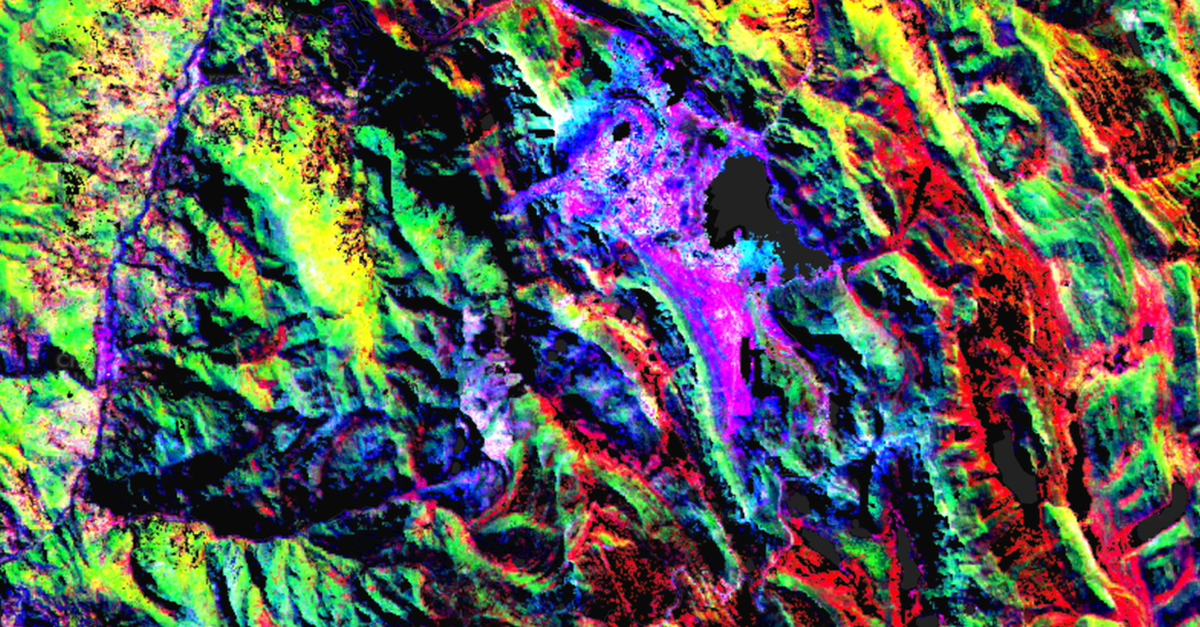
In the conclusion to our Get to Know Marigold series, we compute a Principal Component Analysis,...
Article category: Mining
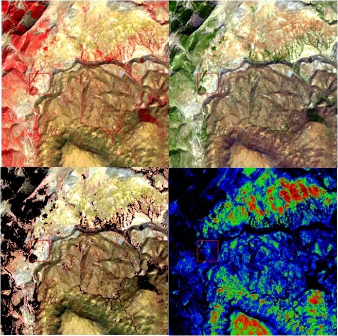
In this blog, we will walk through how to create and deploy vegetation and water masks using the...
Article category: Mining
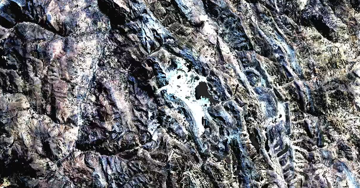
In this blog, we will walk through how to create a series of standard multispectral derived...
Article category: Mining
In this blog, we continue our exploration of Marigold's Workflows & Derived Products on creating...