Get to Know Marigold (Part 7): Marigold Workflows & Derived Products, 3 of 3

Welcome to Marigold. This is part 7 of our Get to Know Marigold blog series with helpful videos. Previous blog series can be found here. Part 1: Functionality and Processing Tools | Part 2: Introduction to the Bare Earth Composites | Part 3: Vegetation and Water Masking | Part 4: Complex Masking, K-Means Clustering Classification | Part 5: Marigold Workflows & Derived Products, 1 of 3 | Part 6: Marigold Workflows & Derived Products, 2 of 3.

This is our final blog in the series and on creating standard multispectral derived products in Descartes Labs’ Marigold software. In the following video snippets , you will learn to create a series of transforms and a basic Spectral Similarity Product. 

The workflows in this video require that you have already masked your data as shown in our Simple and Complex masking videos, as well as created the derived products as shown in Marigold Workflows and Derived Products, 1 of 3 and 2 of 3. Please watch those videos above (Part 3, 4, 5, and 6) before continuing.

Video: Creating a Principal Component Analysis

Let's dive into how we will compute a Principal Component Analysis, which is computed in the same way as a Minimum Noise Fraction Analysis.

Principal Component Analysis (or P-C-A) is a statistical computation that computes the variance in the input dataset, and outputs it as eigenvectors and eigenvalues that are a measure of this variance. Minimum Noise Fraction (or M-N-F) is very similar to P-C-A, the primary difference is that the output components are sorted in the order of noise. For both PCA and MNF, a transform's input bands and output components are always equal in number.

Since both PCA and MNF are computed in the same way, we will only demonstrate the PCA transform in this video. Here’s how to do that in Marigold.

In the Marigold processing toolbox, expand Transforms and select Principal Components Analysis.

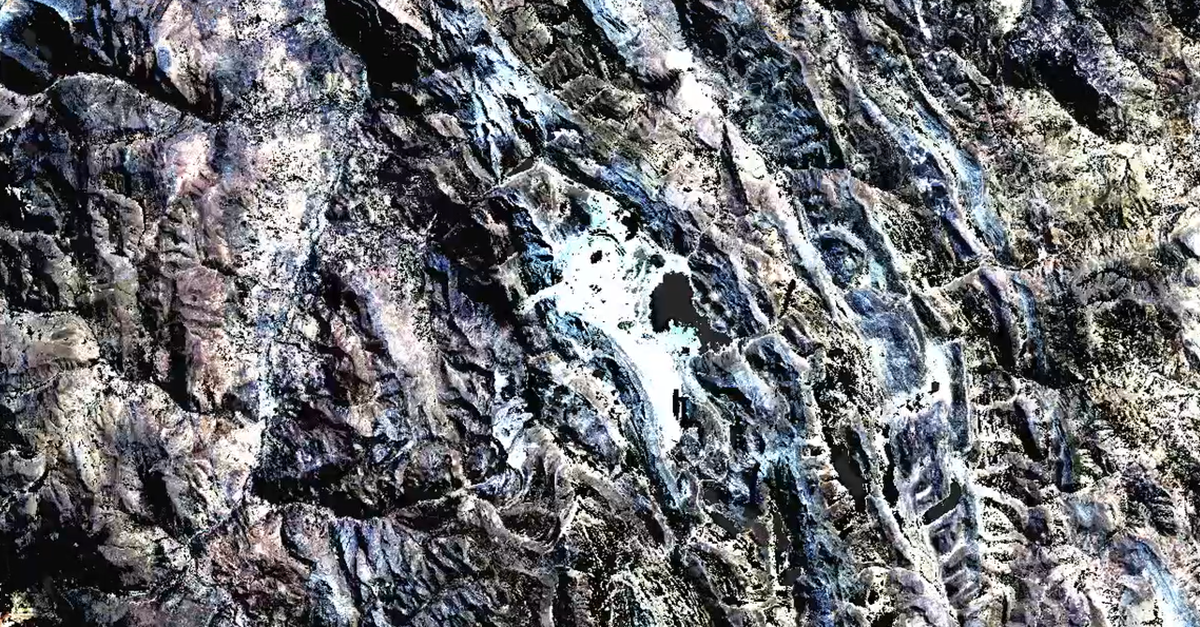
Select your dataset, in this case the masked Fused imagery.  It’s important to use masked input data. Otherwise, the PCA will likely select any unmasked water, vegetation, or other significant factors in the viewport as the initial components. This will not generate the desired results. Select the bands you want to use. Then, provide a relevant name. Finally, click “Run PCA” to generate results.

Video: Changing PCA Output Bands

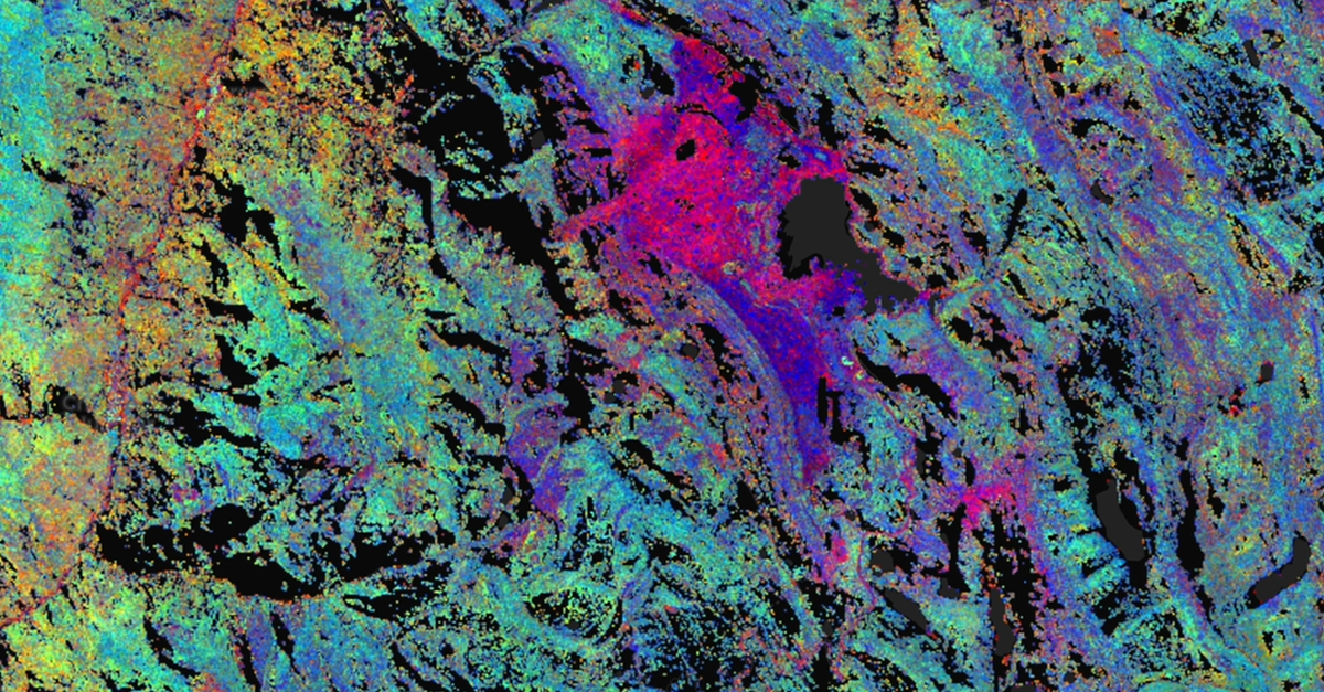
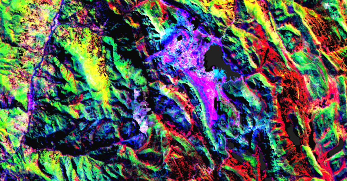
The initial product generated will be a (P-C-A-1, P-C-A-2, P-C-A-3) R-G-B. However, there are many more components to choose from, so we recommend that you verify other components. Often this helps determine which surface cover feature is being selected by each PCA band. To verify, click the three-dot menu on the product layer and select Settings.  You can either examine  single bands, or you can change the component mapped to each band in the RGB product. Let’s change our selection to P-C-A-2, P-C-A-3, and P-C-A-4.  Rename the layer to match the changes, and then click Apply. Click the magic wand on the layer to perform a contrast stretch on the image. 

Note: if the product is switched to a single band, this will automatically apply a colormap, which can be adjusted for a different colormap (i.e. grayscale).  

Video: Creating an Minimum Noise Fraction

With both P-C-A and M-N-F, each of the colors is representing a surface cover type with the same composition - color is a proxy for composition. These two tools are very strong and useful for lithological mapping. For the spatial resolution of the Fused Bare Earth Composite, this differentiation is often used to update geological maps of approximately “one-to-fifty thousand” or higher.

Video: Spectra - Turning on Spectral Query

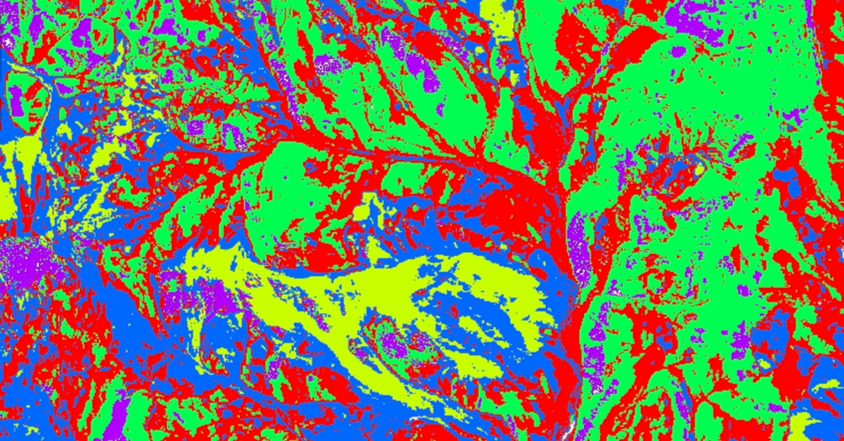
Now let’s explore one of our Supervised Classification Tools. We will create a “Spectral Similarity” product, an interpretation that highlights areas of similar composition.

First, you need to select an “in-scene” spectra of the composition we are trying to match. In Marigold, scroll down beneath the Raster Layers on the left side. In the section called “Spectra,” click the plus sign to expand the menu options. For information on all of the available spectral tools, please refer to our knowledge base article. For our purposes, select “Query Imagery.”

In the product drop-down, select the masked Fused Bare Earth Composite. Select the VNIR bands and the SWIR bands, both which are in units of Surface Reflectance. Do not select the TIR bands, which are in units of Brightness Temperature.

Click “Add Spectral Query.”

Video: Spectra - Picking an In-Scene Spectra

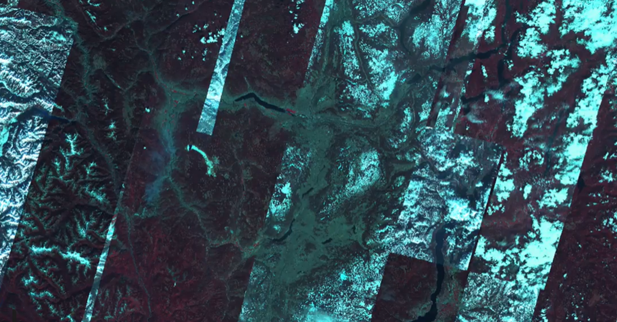
In this location, we will select the “ASTER 641 equivalent” layer to help guide our selection. Once selected, you will see a plus cursor in the viewport. Zoom and click on a location (or composition) of interest. In our example, we will select a ‘purple’ location on the side of the Antamina pit.

Scroll down to see the generated “in-scene” spectra. Its composition is pulled from all of the wavelengths across the Visible Near Infrared, to the Short Wave Infrared. Click and drag on the spectral plot to zoom in on a region you are interested in.

In this plot showing Reflectance versus Wavelength, there is an inflection down, also known as an ‘absorption feature,” at 21-65 nanometers and 22-0-7 nanometers. These each represent the center band positions of ASTER band 5 and ASTER band 6. Absorption features at these positions are both of interest and often indicative of the presence of hydrothermal minerals.

Video: Spectra - Creating a SAM

Next we are going to use these spectra to map locations where the pixels are similar in composition to what we are looking at for this deposit type. 

In the Marigold processing toolbox, expand Classification and select Spectral Angle Mapper, also known as the “SAM” algorithm.

For the input data product, select the masked Fused Bare Earth Composite.  Select the VNIR and SWIR bands. Then select the Spectra that we just generated.  Then, label the output product appropriately. Finally, click “Run SAM”.

Video: Spectra - Adjusting SAM Output

The initially-generated SAM product requires thresholding to improve precision. Locate the layer we just created and click the three-dot menu. Select Settings. Scroll down in the settings window and select “Calculate Histograms''. This creates a detailed histogram of the distribution of the pixel values for this product. 

Hover your mouse at any point on the graph to show the data point information. You can use this to manually set the minimum and maximum values.

To adjust your threshold to the appropriate values, select a minimum value near the middle of the plotted distribution and a maximum value approximately where the distribution approaches the bottom line. 

Click Apply to save your settings.

In the viewport, explore the data to see where the pixels in the pit and the surrounding ground are similar in composition.  This is a very useful, easy-to-make product that can be used to guide brownfields exploration around an existing deposit.

This concludes our Get to Know Marigold blog series on producing remote sensing derived products in Marigold. Thank you for following along on this journey with us. We hope that you have found it useful and can see how Marigold can be applied to your exploration workflows. 

Interested in our Marigold product? Connect with Sales to schedule a consultation.