Article category: Mining
Exciting New Features of Marigold 2.1.0
This article highlights the exciting new user-requested features that are now available in the...
For a fun piece to chew on during the Thanksgiving holiday, National Geographic asked Descartes Labs if we could figure out a way to map every cranberry bog in the United States. We had less than a week to complete the project end-to-end, but we were fortunate to have some pre-existing algorithmic work and data products to consult, which gave us a huge head start.
In the end, the project proved to be a fun and unique problem to solve from a remote sensing perspective. Here, we’ll unpack how we actually did it!
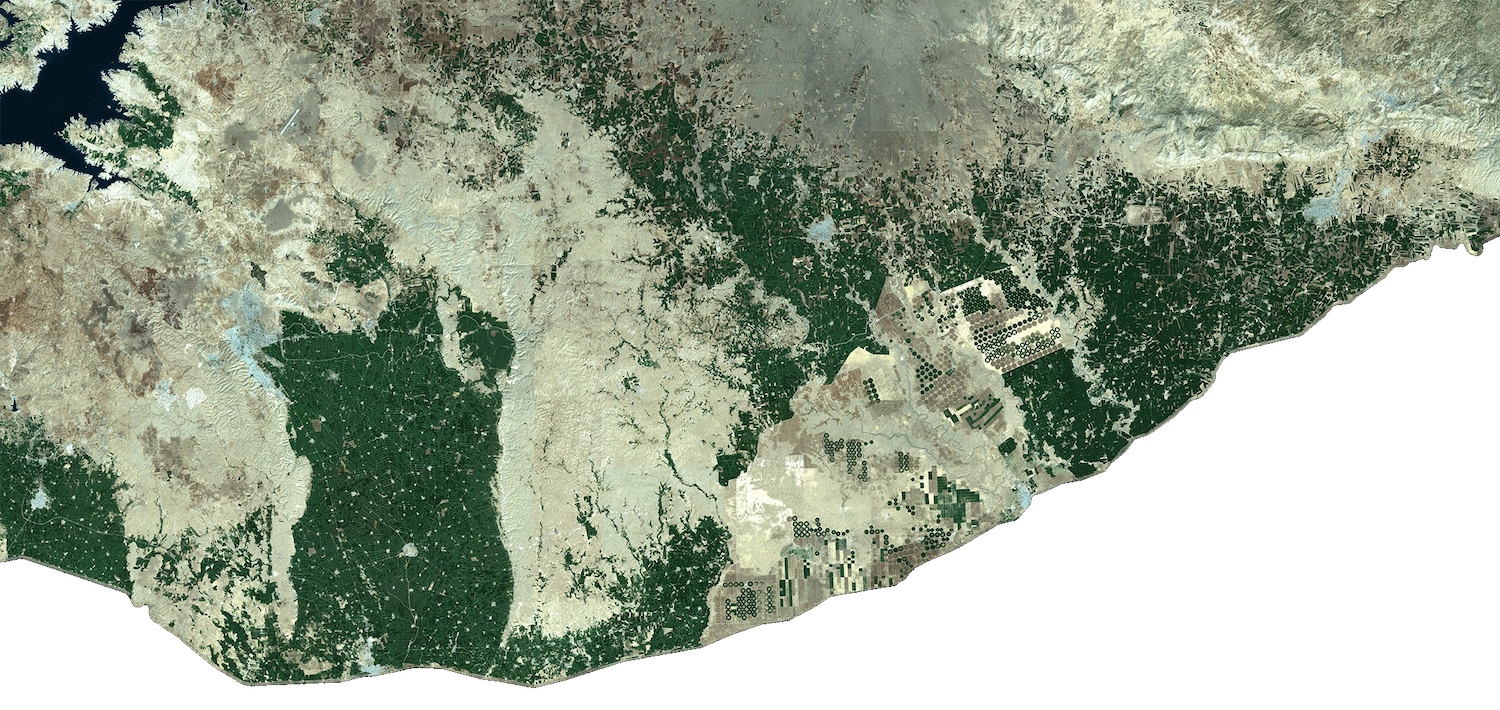
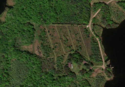
While it sounds simple, it turns out that identifying cranberry bogs from satellite imagery is actually quite tricky. Depending on the time of year, they might look like ponds, bare earth, or lush, green agriculture (like corn)!
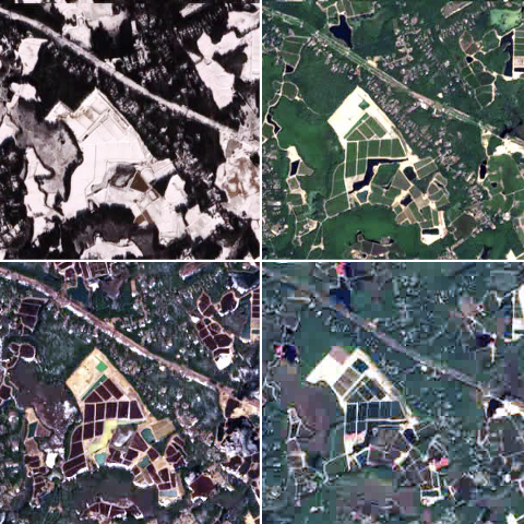
Unless they’re dry harvested, most cranberry bogs in North America are manually flooded before harvest. Unfortunately, the timing of the flooding has enough variability from region to region that we couldn’t get away with simply selecting a single moment in time that would allow us to identify the unique optical imagery signature that indicates a flooded bog.
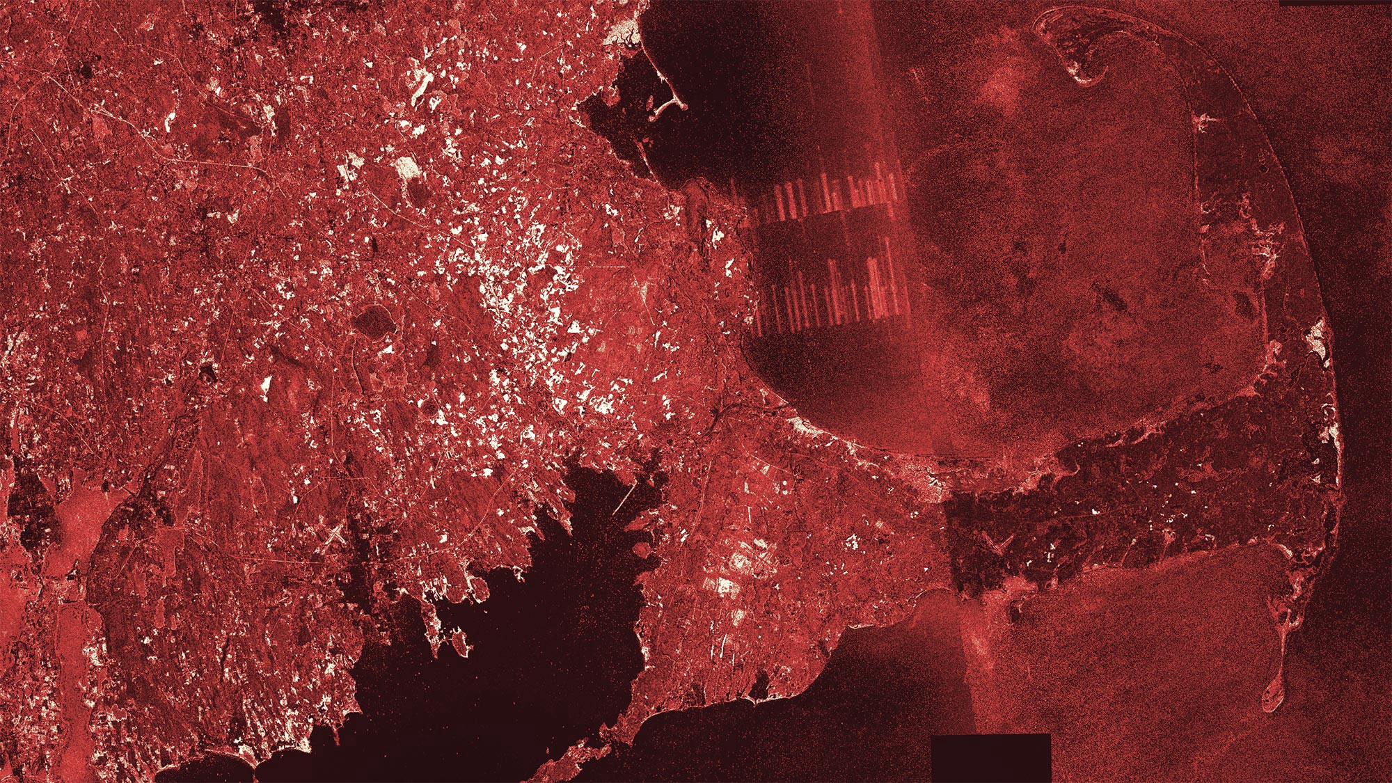
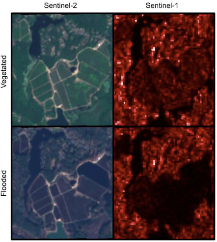
However, what we could do was take advantage of the manual, pre-harvest floods that inundate these bogs by analyzing their signature in synthetic aperture radar (SAR) imagery, which is particularly sensitive to water content.
After analyzing the flood signature in radar imagery, we leveraged techniques we’d used in a previous Descartes Labs project that involved using radar data to map rice paddies — which are also periodically flooded — in Southeast Asia, and combined those with information available to us through the Descartes Labs platform that provides an annual composite of Sentinel-1 radar data, which — critically — includes annual statistics computed from raw amplitude backscatter data. These changes in backscatter represent multiple states in the lifecycle of a cranberry bog. Without this groundwork in place, we most likely would not have been able to accommodate the very short turn-around time for this project.
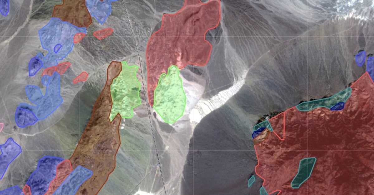
Since temporally aggregated radar statistics are a somewhat abstract way to represent bogs, we applied machine learning to these data sets to find a decision surface that accurately separates the positive (cranberry bog) and negative (not a cranberry bog) class. For the positive class, we were able to locate several active cranberry bogs by scraping data from the GIS departments of Wisconsin, New Jersey and Massachusetts, which, as the top producers of cranberries in the U.S., thankfully make this information freely available.
Picking samples for the negative class ended up being deceptively challenging because sampling from the most ideal regions also risked confusing the classifier. However, sampling a representative set of locations for the negative class is quite important, particularly when dealing with geospatial data, because the machine learning algorithm will otherwise not generalize very effectively. Put another way, teaching the algorithm what isn’t a cranberry bog is just as important as teaching it what is a cranberry bog.
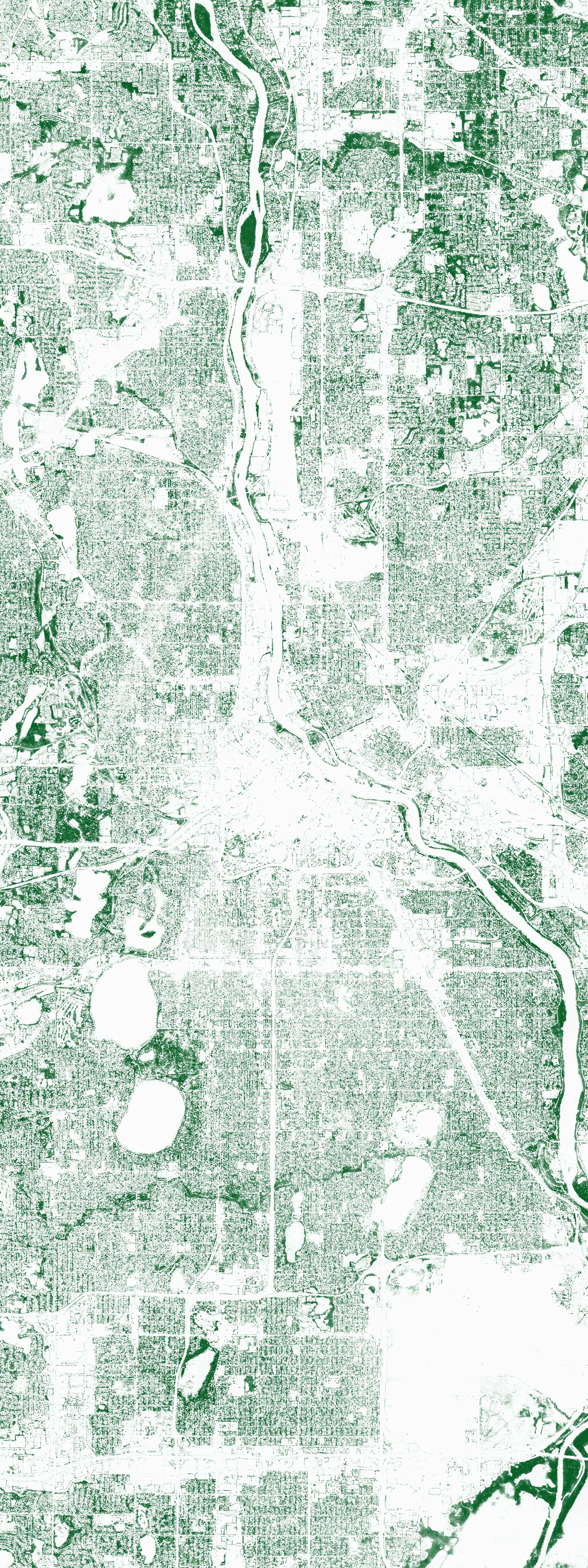
We ended up sampling seven classes from the National Landcover Database (NLCD), ranging from urban areas, to cropland, to wetlands. Finally, we were careful to also sample this data in states with no cranberry bogs to ensure we didn’t incorrectly sample bogs in the negative class.
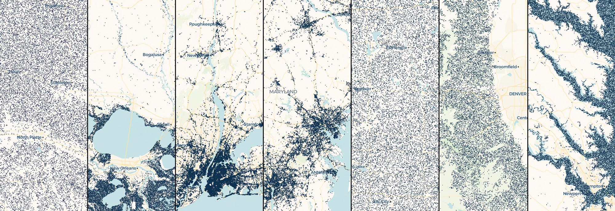
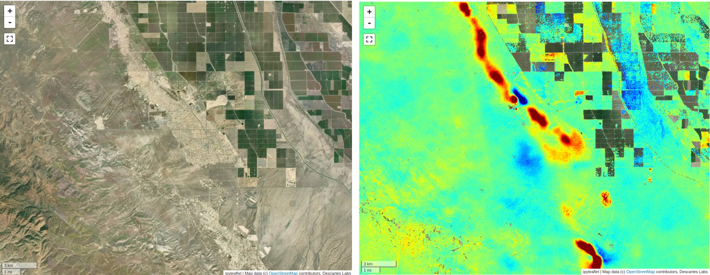
Next, we used our Sentinel-1 annual composite to retrieve the temporal statistics (e.g., min, max, mean, standard deviation) for each location. These statistics were formed into a feature vector on a per-sample basis, and fed into a random forest machine learning classifier. Once trained, given an arbitrary input image of SAR statistics, the model computed the probability of each pixel belonging to a cranberry bog. We leveraged the Descartes Labs platform cloud infrastructure to run this model across all cranberry-producing states and Canadian provinces in a matter of hours.
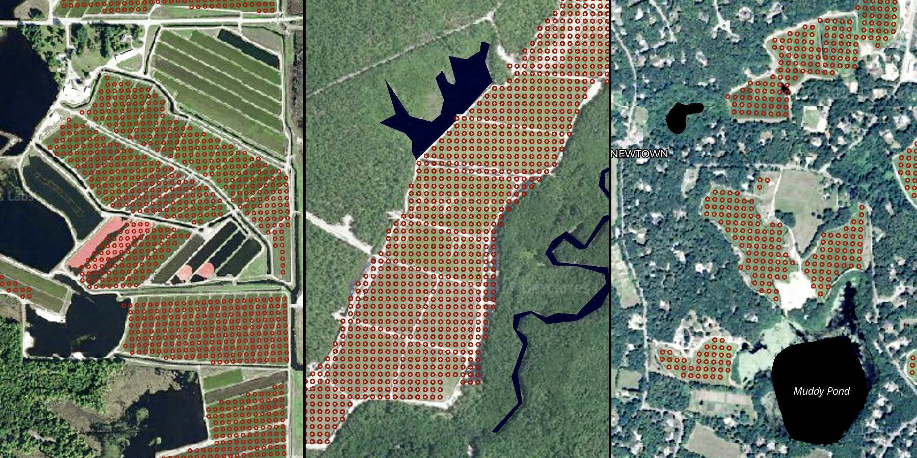
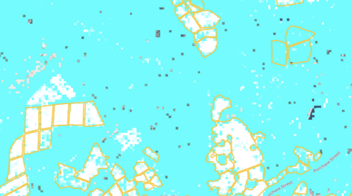
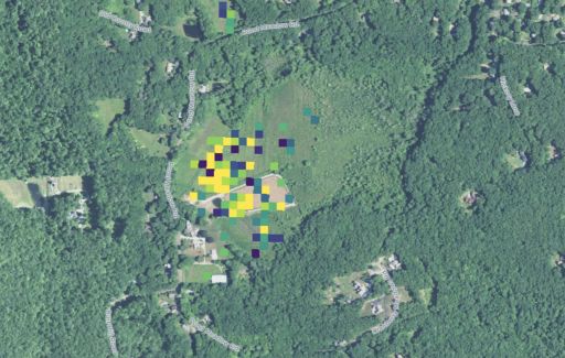
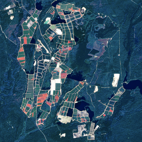
The detector performs quite well! After manually inspecting the probability output, we determined that the detector consistently located every cranberry bog that can be identified by the human eye.
The following set of visuals show a few more interesting discoveries that we made while analyzing the model’s output.
We’re grateful to all the hardworking cranberry farmers in North America, to National Geographic for challenging us with this project, and to our colleagues at Descartes Labs who built the platform that allowed us to rise to the occasion. Who knew that rapid access to petabytes of analysis-ready data and integration, coupled with a vast array of open-source Python packages, would allow us to visualize a holiday staple in a whole new way?
If you’d like to learn more about the Descartes Labs platform and how it could help your work, please contact us here.
Happy Thanksgiving!